Return to Answer

EDIT:

You could use the weight approach above but I also discovered much simpler one. If you are just fine assuming prices can be continuous (which from point of economic theory is fine 0.01c is really just practical limit in real life), then what you can do is skip the creation of deltas at the start:

import numpy as np
import matplotlib.pyplot as plt
buyers = [3.25 - 0.25*n for n in range(0, 11)]
sellers = [3.25 - 0.25*n for n in range(0, 11)] 

Next what you can do is to replace random.choice() with some distribution that has most mass at zero - like the exponential distribution. In python this can be done using random.exponential(), the code would thus change only minimally, and will generate deltas that are closer to the actual valuation of the traders:

trading_prices = []
trading_counts = []

for _ in range(5):
    buyers_still_in_market = list(range(len(buyers)))
    sellers_still_in_market = list(range(len(sellers)))

    transactions = []

    for _ in range(1000):
        # First, a random buyer offers to buy at some price below their number on
        # their card
        b = np.random.choice(buyers_still_in_market)
        delta = np.random.exponential(400)
        buyer_price = max(0, buyers[b] - abs(delta))
        s = np.random.choice(sellers_still_in_market)
        if buyer_price >= sellers[s]:
            transactions.append((b, buyers[b], s, sellers[s], buyer_price))
            buyers_still_in_market.remove(b)
            sellers_still_in_market.remove(s)
            trading_prices.append(buyer_price)

        # Then, a random seller offers to sell at some price above their number on
        # their card. #0.65 - for log normal
        s = np.random.choice(sellers_still_in_market)
        delta = np.random.exponential(400)
        seller_price = sellers[s] + abs(delta)
        b = np.random.choice(buyers_still_in_market)
        if seller_price <= buyers[b]:
            transactions.append((b, buyers[b], s, sellers[s], seller_price))
            buyers_still_in_market.remove(b)
            sellers_still_in_market.remove(s)
            trading_prices.append(seller_price)

    trading_counts.append(len(trading_prices))

    print(len(transactions), "transactions")

plt.plot(list(range(len(trading_prices))), trading_prices)
plt.ylim(0, 4.00)
for x in trading_counts:
    plt.axvline(x=x-1, ymin=0, ymax=4.0, color='red')
    print("line drawn at x =", x)
plt.show()

print(trading_prices)

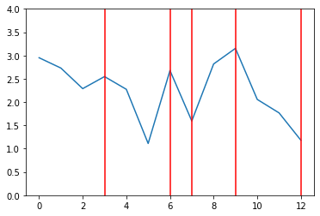
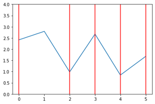
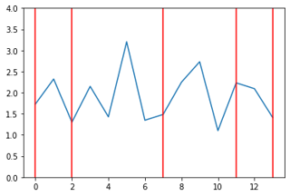
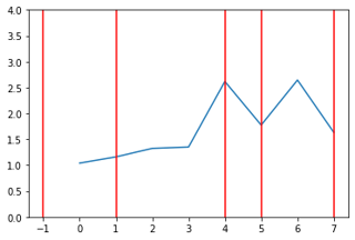
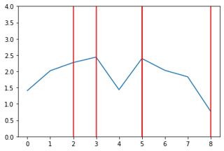
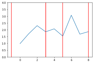
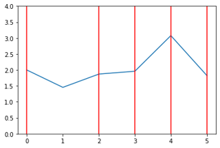
This new code produces results that are much less 'jagged'. Here are some examples, of behavior of price with the exponential distribution (possibly different types of distribution would yield better result but its beyond scope of SE answer to examine that). For example, here are 8 graphs generated when the prices depend on exponential distribution:

I suspect that the reason for that result is the way how you modeled the situation is by having the prices to be offered at random from a sample of numbers in uniform fashion (unless I am misreading the code) but this is unrealistic.

As mentioned in the paper Smith's 1962:

each sequence of experiments was conducted over sequences five to ten minutes long

So the students had only 5-10 minutes to actually conclude the trades. Students knew their own valuation of the item and they wanted to get it.

In such situation it is not in students interest to just choose random price from the sample of prices. Rather students will be choosing from some distribution that will have more mass closer to the their own valuation.

My prediction is that if instead of random sampling of prices from the array you will let the program generate numbers from some distribution that has more mass closer to the right price you will see less volatility in the data.

For example, instead of using random.choice() you could use random.choices() that allows you to assign weights to numbers so some are more likely than others.

I suspect that the reason for that result is the way how you modeled the situation is by having the prices to be offered at random from a sample of numbers in uniform fashion (unless I am misreading the code) but this is unrealistic.

As mentioned in the paper Smith's 1962:

each sequence of experiments was conducted over sequences five to ten minutes long

So the students had only 5-10 minutes to actually conclude the trades. Students knew their own valuation of the item and they wanted to get it.

In such situation it is not in students interest to just choose random price from the sample of prices. Rather students will be choosing from some distribution that will have more mass closer to the their own valuation.

My prediction is that if instead of random sampling of prices from the array you will let the program generate numbers from some distribution that has more mass closer to the right price you will see less volatility in the data.

For example, instead of using random.choice(price_deltas) you could use random.choice(price_deltas, p=weights) that allows you to assign weights to numbers so some are more likely than others.

I suspect that the reason for that result is the way how you modeled the situation is by having the prices to be offered at random over some random sample of numbers in uniform fashion (unless I am misreading the code) but this is unrealistic.

As mentioned in the paper Smith's 1962:

each sequence of experiments was conducted over sequences five to ten minutes long

So the students had only 5-10 minutes to actually conclude the trades. Students knew their own valuation of the item and they wanted to get it.

In such situation it is not in students interest to just choose random price from the sample of prices. Rather students will be choosing from some distribution that will be have more mass closer to the their own valuation.

My prediction is that if instead of random sampling of prices from the array you will let the program generate numbers from some distribution that has more mass closer to the right price you will see less volatility in the data.

For example, instead of using random.choice() you could use random.choices() that allows you to assign weights to numbers so some are more likely than others.

I suspect that the reason for that result is the way how you modeled the situation is by having the prices to be offered at random from a sample of numbers in uniform fashion (unless I am misreading the code) but this is unrealistic.

As mentioned in the paper Smith's 1962:

each sequence of experiments was conducted over sequences five to ten minutes long

So the students had only 5-10 minutes to actually conclude the trades. Students knew their own valuation of the item and they wanted to get it.

In such situation it is not in students interest to just choose random price from the sample of prices. Rather students will be choosing from some distribution that will have more mass closer to the their own valuation.

My prediction is that if instead of random sampling of prices from the array you will let the program generate numbers from some distribution that has more mass closer to the right price you will see less volatility in the data.

For example, instead of using random.choice() you could use random.choices() that allows you to assign weights to numbers so some are more likely than others.