5
$\begingroup$

Suppose there is a linear demand function $D(p)$ describing the demand of an individual consumer. This is derived from a utility function or is just observed, but let us assume it is correct. Now suppose that the product is available at price $p$, but the store insists that each consumer buys a minimum amount that is in fact larger than $D(p)$, but only by very little.
Say it is $D(p) + \epsilon$, where $\epsilon < D(p)/100$.

Can I say without additional assumptions that given the options of buying a quantity $q$ where $q \in \left\{0\right\} \bigcup \left[D(p) + \epsilon,\infty\right)$, the consumer will choose to buy $D(p) + \epsilon$?

My argument is that this will maximize her consumer surplus given the constraint on $q$. As I specified that this is a linear demand function and $\epsilon < D(p)/100$ you can do the math, but it is easy to see that the surplus will be positive for any continuous demand function given a small enough $\epsilon$.

Is this an accepted line of argumentation?

In most models it is accepted that consumers seek to maximize their utility. I am not sure however if one can argue absent a utility function that surplus maximization is the goal.
A workaround would be specifying a quasi-linear utility function supporting $D(p)$ but I would like to avoid this if possible.

$\endgroup$
5
  • $\begingroup$ It is not clear what the consumer’s objective is: max u(.) or CS. If max u(.), I can think it is possible the consumer finds buying 0 quantity making her better off. Consider airline industry. Suppose you are an economy class person but your airline insists that you buy an economy+plus seat which is $125 more expensive. If you are a utility maximizer and find it distasteful that the airline is exploiting you by forcing you to have that extra leg room when you don’t need it, you might be worse off by buying the that e-plus tix. $\endgroup$ Commented Nov 26, 2017 at 3:04
  • $\begingroup$ Now if you buy 0 tix, you don’t get to go where u wanna go, so you might be significantly worse off, thus in this case, you might be forced to buy a strictly positive amount of tix regardless. $\endgroup$ Commented Nov 26, 2017 at 3:06
  • 1
    $\begingroup$ But if she has an alternate transportation means, buying 0 coerced e-plus tix as opposed to renting a car or train or waiting another day (flexible date reservation) may yield a higher payoff. $\endgroup$ Commented Nov 26, 2017 at 3:07
  • $\begingroup$ As to whether a similar example maximizes her CS would follow a similar line of reasoning. How do you define max CS? Making the gap between the willing to price and what u actually pay the biggest? Then, assuming you have to air travel, under your q constraint, in my example, both CS and u-max problem would yield the minimum possible strictly positive quantity optimal. $\endgroup$ Commented Nov 26, 2017 at 3:11
  • $\begingroup$ @FrankSwanton I like your comment about alternate transportation, but I am unsure if this information is not represented already in the demand function. E.g. if there are substites the demand function will be much more price sensitive than if there are none. If you can write up a rigorous (numerical example based) answer where given everything the demand function is truly just a function of price and yet the optimal constrained choice in some sense is not my $D(p) + \epsilon$ I would be happy to accept. $\endgroup$
    – Giskard
    Commented Nov 26, 2017 at 10:55

2 Answers 2

4
$\begingroup$

In a two-good space, initially the consumer maximizes $U(x,z)\;\; s.t. \;\;p_xx+p_zz =I$ and we assume it obtains the solution $(x^*, z^*)$ as a function of prices and income.

In the constrained case, the consumer will either choose $(0, \tilde z)$ or $(x^*+\epsilon, z'$), for some $\epsilon >0 $ always exhausting its budget, so in particular, $\tilde z = I/p_z$. In order for the consumer to still choose to buy a strictly positive quantity of $x$, it must be the case that

$$U(x^*+\epsilon, z') > U(0, \tilde z)$$

Apply a first order approximation around $(x^*, z^*)$ without ignoring the remainders, we want

\begin{align} U(x^*, z^*) + U_x(x^*)\cdot \epsilon + U_z(z^*)(z'-z^*) + R_{\epsilon} &\\> U(x^*, z^*) + U_x(x^*)(-x^*) + U_z(z^*)(\tilde z-z^*) + R_0 \end{align}

Simplify and re-arrange, we want

$$U_x(x^*)(x^*+\epsilon) + R_{\epsilon} > U_z(z^*)(\tilde z-z') + R_0 $$

We know that from the unconstrained optimization, $U_x(x^*)/U_z(z^*) = p_x/p_z$ so

$$\frac {p_x}{p_z}(x^*+\epsilon) + \frac {R_{\epsilon}}{U_z(z^*)} > \left(\frac{I}{p_z}-z'\right) + \frac {R_0}{U_z(z^*)} $$

Multiply throughout by $p_z$,

$$p_x(x^*+\epsilon) + p_z\frac {R_{\epsilon}}{U_z(z^*)} > I - p_zz' + p_z\frac {R_0}{U_z(z^*)} $$

but $p_x(x^*+\epsilon) + p_zz' = I \implies p_x(x^*+\epsilon) = I-p_zz'$ so we are left with the requirement that (ignoring positive terms)

$$R_{\epsilon} > R_0 $$

in order for the consumer to choose $x^*+ \epsilon$ and not $0$ for $x$.

Note that the above take into account also the signs of the remainders, it is not just about their absolute magnitudes.

Now let's go back to our first-order expansions. We know that both candidate bundles yield utilities lower than $U(x^*, z^*)$, because they were feasible in the unconstrained case, and they weren't chosen.

Looking at the expansion of $U(0, \tilde z)$ we then conclude that we have

$$U_x(x^*)(-x^*) + U_z(z^*)(\tilde z-z^*) + R_0 < 0 $$

$$\implies U_z(z^*)\cdot \Big[(U_x(x^*)/U_z(z^*))\cdot(-x^*) + \tilde z-z^*\Big] + R_0 < 0$$

$$\implies \frac {U_z(z^*)}{p_z}\cdot \Big[-p_xx^* + p_z\tilde z-p_zz^*\Big] + R_0 < 0$$

But $-p_xx^* -p_zz^* = -I$ and $p_z\tilde z =I$ so the term in brackets is zero. Therefore we conclude that

$$R_0 <0$$

Looking now at the expansion of $U(x^*+\epsilon, z')$, we know we have

$$U_x(x^*)\cdot \epsilon + U_z(z^*)(z'-z^*) + R_{\epsilon} < 0$$

Performing the same manipuations as before we obtain here too that

$$R_{\epsilon} < 0$$

So the condition to buy $x^*+\epsilon$ can be re-written as

$$|R_{\epsilon}| < |R_0|$$

This formalizes somewhat the notion that if $\epsilon$ is "sufficiently small", $R_{\epsilon}$ will be smaller in absolute terms than $R_0$, since the approximation to the same function will be "better", and so we will observe $x^*+\epsilon$ and not $0$. But it also tells us what the graphs in the other answer told us too, that there is not a single general answer to the matter.
$\endgroup$
2
  • $\begingroup$ Very nice walk through, thank you. There is a slight mischief where you assume that the marginal rate of substitution exists in $(x^*,z^*)$ but it is non-essential. It seems that my original question fell to two pieces though. This showed that utility maximization yields the $x^* + \epsilon$ solution as optimal, if $\epsilon$ is small enough. What I would really like to know is if I can make the same claim if there is no explicit utility function, only a demand function. (Given a linear demand function the upper bound on acceptable $\epsilon$ values would probably be $x^*$.) $\endgroup$
    – Giskard
    Commented Nov 27, 2017 at 21:39
  • $\begingroup$ No need to answer part 2 here, I will try to clarify and repost it. $\endgroup$
    – Giskard
    Commented Nov 27, 2017 at 21:41
3
$\begingroup$

It appears that the consumer faces an exogenous additional constraint in her optimization problem, which restricts the feasible set for the good in question, say $x$. We take this for granted: the consumer will buy either zero or at least what the store demands at the minimum, say $\bar x$. No other options are available. But this means that the consumer must solve again her optimization problem, incorporating this additional constraint and its effect on the feasible set - the "initial" demand function is not relevant anymore, because it represents a solution to a problem that has just been altered.

What will the result be?

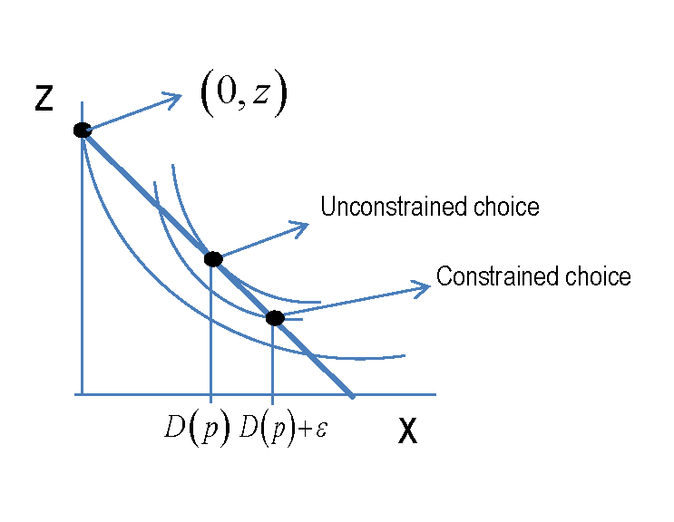
Assuming "usual" preferences, let a two-good utility function $U(x, z)$. then, graphically,

enter image description here

Choosing to buy zero will send the consumer to an even lower utility level, than the one forced on her by the minimum quantity requirement.

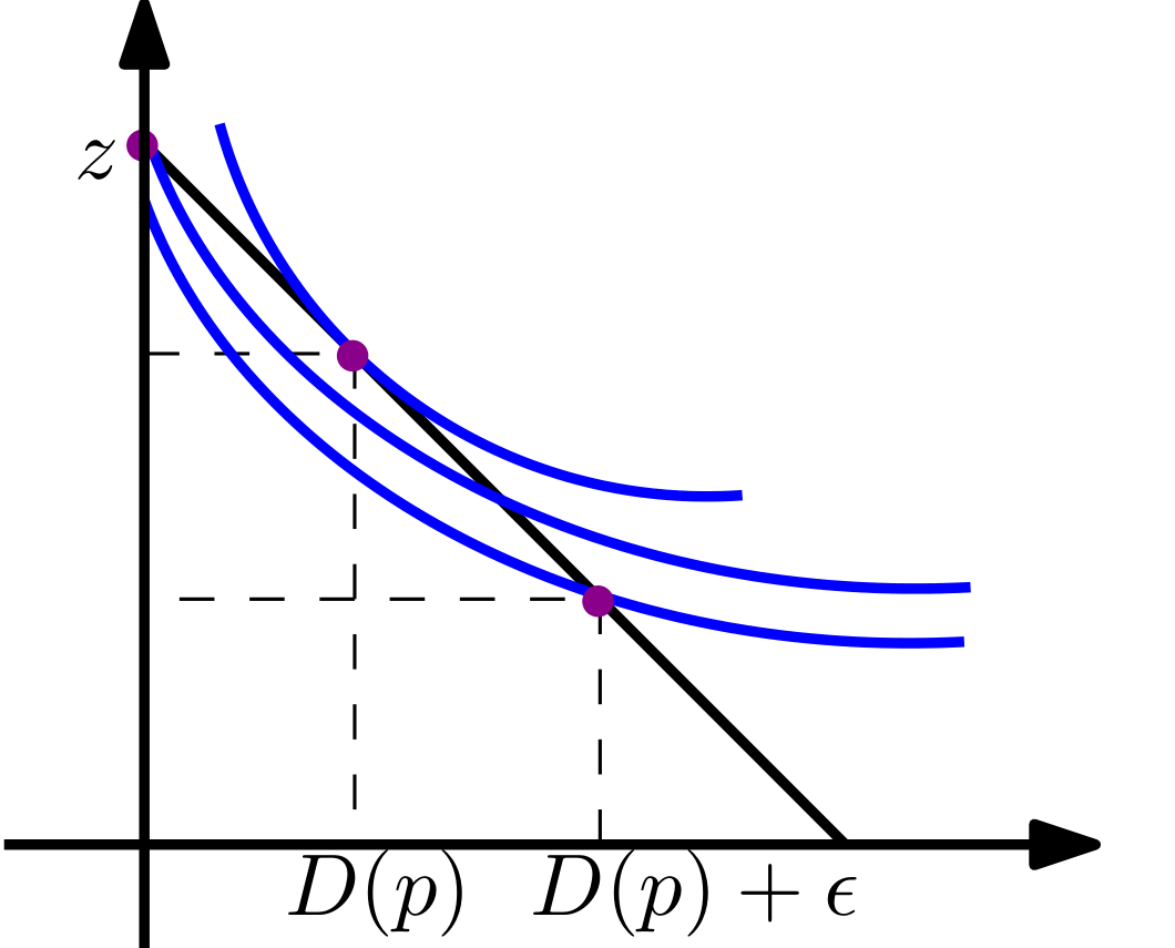
EDIT by denesp: What about this graph though?

enter image description here

RESPONSE : It does tell us what we should expect after all: the smaller the quantity demanded in the unconstrained solution, and the larger the distance of this solution from the minimum quantity required by the store, the more possible it becomes that the consumer will choose to buy zero in the end. So it appears there is no single answer to the general question, even under "usual" preferences. Intuitively of course, if the distance is "very small" and the unconstrained solution is not "very small" to begin with we expect that usual preferences will lead the consumer to buy the bit more that the store requires.

Maybe all this could be made into a rigorous description exploiting the lengths measured on the budget constraint between, the zero bundle and the unconstrained solution, and between the uncostrained solution and the minimum quantity required by the store.

$\endgroup$
10
  • $\begingroup$ I mention not wanting to go the utility function road two times in my question. The question is pretty much "is this info included in the demand function alone"? You say "this means that the consumer must solve again her optimization problem". Why? This is what I would like to know. Isn't $D(p)$ the solution function of the convex unconstrained optimization problem already? $\endgroup$
    – Giskard
    Commented Nov 26, 2017 at 10:47
  • $\begingroup$ Unfortunately even admitting utility functions the graph does not really prove anything. I can easily draw another one where the usual conditions on preferences are fulfilled but the slopes of the indifference curves are manipulated in such a way that $(0,z)$ becomes the optimal constrained choice. $\endgroup$
    – Giskard
    Commented Nov 26, 2017 at 10:49
  • $\begingroup$ @denesp As for the first comment, since the consumer surplus you are examining is based on a demand function that no longer holds, what makes you think that you could get away with it without revisiting the maximization problem? I stated as much in my answer. As for the second comment, probably, but it exceeds my powers of visualization so I would like to see that graph, and what kind of preferences it will reflect. $\endgroup$ Commented Nov 26, 2017 at 10:54
  • $\begingroup$ @denesp Under the new constraint the unconstrained solution is not feasible anymore, so the problem must be resolved, don't you think? $\endgroup$ Commented Nov 26, 2017 at 10:56
  • 1
    $\begingroup$ @denesp I did not post my answer and graph as a proof of your conjecture, but it appears it looks that way... I will leave this answer as is and post another one with the rigorous treatment. $\endgroup$ Commented Nov 26, 2017 at 11:51

Your Answer

By clicking “Post Your Answer”, you agree to our terms of service and acknowledge you have read our privacy policy.

Not the answer you're looking for? Browse other questions tagged or ask your own question.