6
$\begingroup$

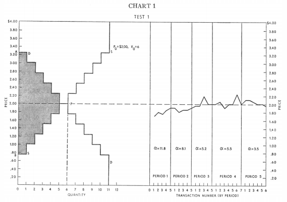
Vernon Smith's 1962 paper "An Experimental Study of Competitive Market Behavior" simulates a market using students (who have piece of paper giving their reservation prices). In one of the experiments, the demand/supply curves look like the graph on the left, with the corresponding market activity on the right:

chart 1 from Smith's paper

Since there seems to be nothing special about using students in the experiment (i.e. as far as I can tell, they are just performing simple computations), I decided to code up the experiment in Python. My script is here.

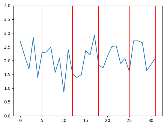
When I run the script (which has the same demand/supply curves as above), the market activity typically looks like this:

my plot

The market price does indeed hover around $2.00, but my graph seems noticeably more jagged than the graph in the original paper. I'm trying to figure out what's going on, in particular whether:

  1. I'm understanding the paper incorrectly somehow, or
  2. My Python script has some error in it, or
  3. There's some kind of error or unwritten assumption in the paper.
$\endgroup$
3
  • 1
    $\begingroup$ I'm not an expert in parsing Python codes, but I suspect that the particular decision/trading algorithm(s) was the reason for the sustained volatility. It would help if you could describe verbally the decision algorithms in your script. $\endgroup$
    – Herr K.
    Commented Feb 9, 2021 at 2:52
  • $\begingroup$ May be renamed "reproducing distribution" instead of "understanding" to get more specialist feedback. $\endgroup$ Commented Feb 9, 2021 at 10:43
  • $\begingroup$ one can only answer question that was being asked not question that was meant to be asked - that does not make feedback any less specialist - this being said I made some adjustment to your code that reduced the 'jaggedness' - however, as the HerK answer explain there is not much you can do with pure random trading - an alternative would be to specify the agents through some model + AI/learning algorithm - however that is too time consuming to code it all from nothing for an SE answer $\endgroup$
    – 1muflon1
    Commented Feb 9, 2021 at 16:33

3 Answers 3

3
$\begingroup$

I suspect that the reason for that result is the way how you modeled the situation is by having the prices to be offered at random from a sample of numbers in uniform fashion (unless I am misreading the code) but this is unrealistic.

As mentioned in the paper Smith's 1962:

each sequence of experiments was conducted over sequences five to ten minutes long

So the students had only 5-10 minutes to actually conclude the trades. Students knew their own valuation of the item and they wanted to get it.

In such situation it is not in students interest to just choose random price from the sample of prices. Rather students will be choosing from some distribution that will have more mass closer to the their own valuation.

My prediction is that if instead of random sampling of prices from the array you will let the program generate numbers from some distribution that has more mass closer to the right price you will see less volatility in the data.

For example, instead of using random.choice(price_deltas) you could use random.choice(price_deltas, p=weights) that allows you to assign weights to numbers so some are more likely than others.


EDIT:

You could use the weight approach above but I also discovered much simpler one. If you are just fine assuming prices can be continuous (which from point of economic theory is fine 0.01c is really just practical limit in real life), then what you can do is skip the creation of deltas at the start:

import numpy as np
import matplotlib.pyplot as plt
buyers = [3.25 - 0.25*n for n in range(0, 11)]
sellers = [3.25 - 0.25*n for n in range(0, 11)] 

Next what you can do is to replace random.choice() with some distribution that has most mass at zero - like the exponential distribution. In python this can be done using random.exponential(), the code would thus change only minimally, and will generate deltas that are closer to the actual valuation of the traders:

trading_prices = []
trading_counts = []

for _ in range(5):
    buyers_still_in_market = list(range(len(buyers)))
    sellers_still_in_market = list(range(len(sellers)))

    transactions = []

    for _ in range(1000):
        # First, a random buyer offers to buy at some price below their number on
        # their card
        b = np.random.choice(buyers_still_in_market)
        delta = np.random.exponential(400)
        buyer_price = max(0, buyers[b] - abs(delta))
        s = np.random.choice(sellers_still_in_market)
        if buyer_price >= sellers[s]:
            transactions.append((b, buyers[b], s, sellers[s], buyer_price))
            buyers_still_in_market.remove(b)
            sellers_still_in_market.remove(s)
            trading_prices.append(buyer_price)

        # Then, a random seller offers to sell at some price above their number on
        # their card. #0.65 - for log normal
        s = np.random.choice(sellers_still_in_market)
        delta = np.random.exponential(400)
        seller_price = sellers[s] + abs(delta)
        b = np.random.choice(buyers_still_in_market)
        if seller_price <= buyers[b]:
            transactions.append((b, buyers[b], s, sellers[s], seller_price))
            buyers_still_in_market.remove(b)
            sellers_still_in_market.remove(s)
            trading_prices.append(seller_price)

    trading_counts.append(len(trading_prices))

    print(len(transactions), "transactions")

plt.plot(list(range(len(trading_prices))), trading_prices)
plt.ylim(0, 4.00)
for x in trading_counts:
    plt.axvline(x=x-1, ymin=0, ymax=4.0, color='red')
    print("line drawn at x =", x)
plt.show()

print(trading_prices)

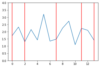
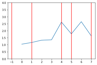
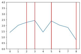
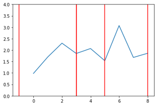
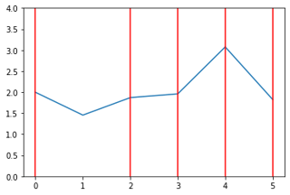
This new code produces results that are much less 'jagged'. Here are some examples, of behavior of price with the exponential distribution (possibly different types of distribution would yield better result but its beyond scope of SE answer to examine that). For example, here are 8 graphs generated when the prices depend on exponential distribution:
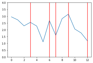
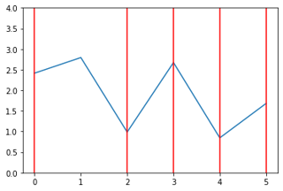
enter image description here enter image description here enter image description here enter image description here enter image description here enter image description here enter image description here enter image description here

$\endgroup$
2
  • $\begingroup$ Thanks! I feel convinced that it is indeed the way the deltas are chosen that is causing the jaggedness. When I use exponential deltas though, the trading prices seem to still range around 1.5 to 2.5, the same as my original graph. I think the reduced jaggedness in your graph is coming not from prices being more stable around the equilibrium price, but instead from there being fewer trades (there's not much room to be jagged when only 2-3 trade are made in a single period). $\endgroup$
    – IssaRice
    Commented Feb 10, 2021 at 21:21
  • $\begingroup$ @riceissa I did not save the further output, but I know for sure volatility of prices dropped because I actually calculated the volatility of prices based on the list at the end, compared it to the original and, and it was lower in this new one than in original script. $\endgroup$
    – 1muflon1
    Commented Feb 10, 2021 at 21:27
4
$\begingroup$

Gode and Sunder (1993) recorded a result similar to yours. The abstract of the paper reads:

We report market experiments in which human traders are replaced by "zero-intelligence" programs that submit random bids and offers. Imposing a budget constraint (i.e., not permitting traders to sell below their costs or buy above their values) is sufficient to raise the allocative efficiency of these auctions close to 100 percent. Allocative efficiency of a double auction derives largely from its structure, independent of traders' motivation, intelligence, or learning. Adam Smith's invisible hand may be more powerful than some may have thought; it can generate aggregate rationality not only from individual rationality but also from individual irrationality.

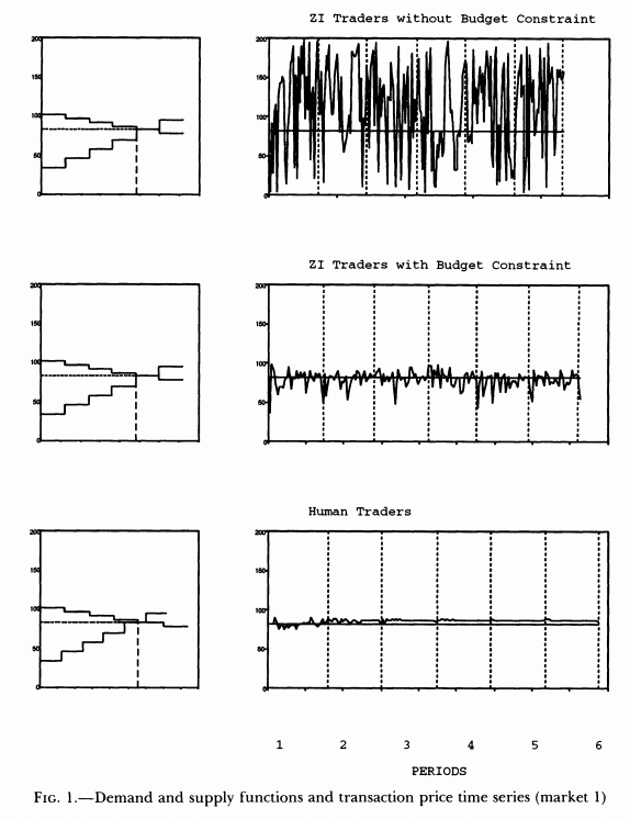
Specifically, Gode and Sunder consider two algorithms of trade. The first algorithm generates bids and asks from a uniform distribution on a fixed interval, say $[L,U]$, irrespective of the traders' reservation values. The authors refer to these traders as unconstrained zero intelligence (ZI-U) traders. In the second algorithm, bids are drawn from $\mathrm{unif}[L,v]$ and asks are drawn from $\mathrm{unif}[c,U]$, where $v,c$ are the reservation values for buyers and sellers respectively. The traders following this second algorithm are referred to as constrained zero intelligence (ZI-C) traders.

The following figure (along with several others in the paper with different market parameters) shows that ZI-U traders generate more sustained price volatility than ZI-C traders, who in turn resemble human traders in the same market condition. So I suspect that the sustained volatility you observed in your code was due to the fact that you used uniform bounds on the random bid/ask generation instead of imposing a budget constraint for the traders.

enter image description here

$\endgroup$
2
  • $\begingroup$ Thanks, I appreciate this reference! (I found Smith's paper mentioned in my econ 101 textbook without any reference to other literature since then, and I am too much of an econ noob to quickly find the relevant papers.) $\endgroup$
    – IssaRice
    Commented Feb 10, 2021 at 21:23
  • 1
    $\begingroup$ @riceissa: You're welcome. You may also refer to Duffy's chapter in the Handbook of Computational Economics for other related developments in the literature. $\endgroup$
    – Herr K.
    Commented Feb 10, 2021 at 22:32
2
$\begingroup$

Smith's human traders adapted their behavior, learning from experience between successive market periods, which is another reason why their transaction-price time-series is so much smoother than yours (or Gode & Sunder's ZIC results).

For a free open-source detailed Python simulation of a financial exchange populated with traders that do adapt over time, learning from experience, see:

https://github.com/davecliff/BristolStockExchange/wiki

Especially the Jupyter notebook here, which is a walkthrough of recreating Smith's 1962 results (his Chart 1 graph) with simulated traders:

https://github.com/davecliff/BristolStockExchange/blob/master/BSE_VernonSmith1962_demo.ipynb

$\endgroup$

Your Answer

By clicking “Post Your Answer”, you agree to our terms of service and acknowledge you have read our privacy policy.

Not the answer you're looking for? Browse other questions tagged or ask your own question.