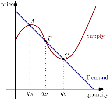
Forgive me in advance if this is already familiar. I'll be talking about stability of equilibrium the way I (briefly) learned it.
Let $\xi^j(p)$ denote the excess demand for good $j$ given price $p$.
$$\xi^j(p) = \sum^m_{h=1}\left( x^j_h(p) - e^j_h \right) = x^j(p) - r^j$$
For $m$ households/consumers, $e$ being an endowment to a household, and $r^j$ being the total resource available of good $j$. We say the rate of price adjustment over time $\left(\frac{\partial p^j}{\partial t}\right)$ is proportional to excess demand.
For either of your market clearing prices $p^*$, we then know that $x^j(p^*) = r^j \ \forall j \implies \xi^j(p) = 0$
Otherwise,
$\xi^j(p)> 0 \implies \text{excess demand} \implies \frac{\partial p^j}{\partial t} > 0$
$\xi^j(p)< 0 \implies \text{excess supply} \implies \frac{\partial p^j}{\partial t} < 0$
Out of the three equilibrium you have up there, we'd probably want to find one that was locally stable and say that's where the market is more likely to realistically go.
Steady state $p^*$ is locally stable if $\exists \epsilon > 0 \ \text{s.t.} \ \forall \ p(0) \in B_\epsilon (p^*)$, an open neighborhood with radius $\epsilon$ around $p^*$, then we have $p(t, p(0)) \rightarrow p^*$
I don't want to fuddle this too much with math (particularly when you linearize the system and have to deal with eigenvalues/eigenvectors), so let's just take a look at your supply and demand curves above. We can peruse the math on our own time.
Case A: Let's say you are at point A, your nice equilibrium. Suddenly there is a downwards quantity shock and you are now to the left of $q_A$. Since there is excess demand, the change in price over time should be positive, so the price will rise, and you will arrive back at point A.
What if you are shocked to the right of $q_A$ in the short run? Now there is excess supply and price over time should fall. If you were still above $p^*_A$ at this point, you will arrive back at point A. Otherwise price will fall all the way until you reach point B.
Case B: We know what happens with a shock to the left of point B now. What about to the right? If point C looks like a global minimum of the supply curve from what it looks like, then any shock that gets you before point C gets you excess demand, which means the price will rise and you will arrive back at point B.
Case C: To the right of point C, there is excess supply, and prices will fall back down until you reach C again.
None of these equilibria seem globally stable. It seems C is not locally stable on the left, so I wouldn't say the market would hang out there for very long. Points A and B are locally stable, but it seems B has greater room to get shocked and still move back towards B.
So for this scenario, I personally like B as your long run equilibrium.
If you had extra information about how shocks in the market happen (how often, variance, etc.), it may allow you to describe what percentage of the time you stick around at each equilibria, and you could describe an aggregate equilibrium like that as well.
