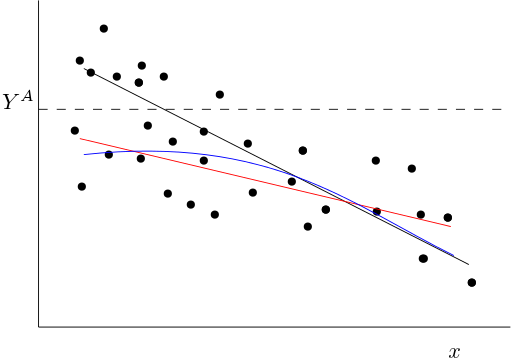
The situation is given in the following picture

The black line is the true conditional mean $E(y|x)$. If we truncate the data, all observations above the truncation $Y^A$ are not observed.
For low values of $x$, we will observe (on average) lower values of $y$ than we would without the truncation. As such, when $x$ is low, the observed conditional mean function (in blue) will be lower than the true one. If you fit a linear function through the observed points (say in red), you will therefore fit a linear function approximating the blue one. This will be a function with a flatter slope (compared to the true conditional mean in black).
The following is not exact, but only gives an idea how I would approach the problem analytically.
Assume that the true data generating process be given by:
$$
y_i = \beta_0 - \beta_1 x_i + \varepsilon_i.
$$
Where, as usual, $E(\varepsilon_i) = 0$ and $E(\varepsilon|x_i) = 0$. The conditional mean function is then equal to:
$$
E(y_i|x_i) = \beta_0 - \beta_1 x_i + E(\varepsilon_i|x_i) = \beta_0 - \beta_1 x_i.
$$
Now let $z_i$ be the random variable equal to 1 iff observation $i$ is not truncated, i.e. when
$$
\beta_0 - \beta_1 x_i + \varepsilon_i < Y^A.
$$
If $i$ is not observed, i.e. truncated, we have $z_i = 0$.
Then the observed conditional mean equals:
$$
E(y_i|x_i,z_i=1) = \beta_0 - \beta_1 x_i + E(\varepsilon_i|x_i, z_i = 1).
$$
The last term is given by:
$$
E(\varepsilon_i|x_i, z_i = 1) = E(\varepsilon_i|x_i, \varepsilon_i < Y^A - \beta_0 + \beta_1 x_i)
$$
This last term, which is a function of $x_i$ is negative (as $\varepsilon_i$ is truncated from above and the mean of the untrunctated $\varepsilon$ is zero). Define:
$$
E(\varepsilon_i|x_i,\varepsilon_i < Y^A - \alpha_0 + \alpha_1 x_i) = g(x_i).
$$
we have that $g(x_i) < 0$ and in general, we would expect that $g'(x_i) > 0$, because the restriction is less binding if $x_i$ becomes bigger (This however is probably not always the case, as $g$ depends on the shape of the joint distribution of $\varepsilon_i$ and $x_i$.)
Then we have:
$$
E(y_i|x_i, z_i = 1) = \alpha_0 + \beta_1 x_i + g(x_i),
$$
This is the blue curve in the picture.
The slope of this line equals:
$$
\frac{\partial E(y_i|x_i, z_i = 1)}{\partial x_i} = -\beta_1 + g'(x_i)
$$
The right hand side of the first equation is bigger than $-\beta_1$ (so the slope is flatter).
Notice that in general, the conditional mean will alsono longer be a linear function of $x_i$, so there will also be a specification bias. This also makes it not trivial to determine what exactly the bias will be from fitting a linear function.
Lowering the value of $Y^A$ will lead to a larger bias (more negative $g(x_i)$) and probably also to a flatter slope of the estimated regression. I hope this is intuitive from the picture above.
