10
$\begingroup$

It's well understood that the cost of living in New York City vastly exceeds the cost of living in, say, rural Louisiana. It is also well understood that wages in New York City vastly exceed those in rural Louisiana. My question is: who comes out ahead?

To clarify, let me offer a thought experiment (not sure if this is valid or not, I'm no economist). Imagine we have two individuals: one in rural Louisiana with a low cost of living and low wage ("Lou" for short), the other in New York City with a high cost of living and a high wage ("Nue" for short). Imagine that both Lou and Nue earn exactly the median household income for their respective region. They live in virtually identical homes (paying the local rent). They drive virtually identical cars. They have the same number of children. They have the same healthcare plan, and so on. Now imagine that each day Lou and Nue both go to the mall, and buy the exact same items as one another (paying the local price). Let's imagine they are spending very quickly, far more quickly than either can afford. Who runs out of money first, Lou or Nue?

A follow up question: is there a single number which tracks this quality I'm trying to describe? It seems like median income divided by local CPI would just about do it, but that's purely based on my own untrained intuition.

$\endgroup$
1
  • $\begingroup$ The averages are misleading. It has to break down on the type of job and the ability of the individual. A high ability bio-chemist and a fast food restaurant worker see very different PPP. $\endgroup$
    – user5308
    Commented Jul 28, 2015 at 5:59

3 Answers 3

10
$\begingroup$

TL;DR Wages offset the high cost of living in most states. In NY and CA specifically, wages are insufficient to offset the high cost of living. In New York City specifically, wages do not even come close to offsetting the high cost of living.

Having now researched this a bit, I can give a very concrete answer to the Lou/Nue hypothetical, and I think a pretty decent answer to the general idea. Let me just say up front, I am not an economist, I'm taking a best guess based on the data published by real economists. These are layman's conclusions, and, as BKay pointed out, can't possibly capture the complexity of the real world. That said...

Nue runs out of money first. Here's why:

The regional price parity (RPP) in NYC is 136. That means, a purchase which costs \$100 for an average American will cost \$136 for an average resident of NYC. The median income in NYC is \$50,711. This is 97% the national median income. This means that a days work which pays \$100 for an average American pays \$97 dollars for an average resident of NYC.

The regional price parity in Louisiana is 91. A purchase which costs \$100 for an average American will cost \$91 for an average resident of Louisiana. The median income in Louisiana is \$40,462. This is 77% the national average. This means that a days work which pays \$100 for an average American pays \$77 dollars for an average resident of Louisiana.

In addition to Lou and Nue, also let us consider Medie. Medie earns exactly the national median income, and her cost of living is exactly the national average, i.e. RPP = RWP = 100. (Sidebar: to the extent that such a person exists, they probably live in Pennsylvania, which comes the closest to conforming to both wage and price averages). So let's compare a hypothetical wage and price for Medie, Lou, and Nue:

Medie earns \$100 per day
Apples cost \$1 each in Medie's home town
Medie can buy 100 apples per day

Lou earns \$77.81 per day
Apples cost \$0.91 each in Lou's home town
Lou can buy 85 apples per day

Nue earns \$97.63 per day
Apples cost \$1.36 in Nue's home town
Nue can buy 71 apples per day

Note, this effect only holds for New York City proper. If you compare New York State with Louisiana, they are dead even.

To answer the question more generally, all other things being equal it pays to be in a high wage, high cost of living state, though there is major regional variation. To try and answer this more fully, let's look at the data BKay supplied above, and expand the hypothetical from the original question. Regional Price Parity data is fairly easy to come by (i.e., "for every dollar spent by an average american, how many dollars must a person from region X spend to get the same result?"). Regional Median Wage data is also pretty easy to come by. From the Regional Median Wage we can trivially calculate Regional Wage Parity (i.e. "for every dollar earned by an average American, how many dollars can a person in region X expect to earn?"). This is a term I'm making up, so I know it's not exactly scientific, but I think it give a good gestalt for the situation. This gives us:

$$ \frac{Regional Wage Parity}{Regional Price Parity} = HowMuchStuffYouCanBuy $$

"How much stuff you can buy" is really the figure that this question is trying to get at.

The state with the highest "apples per day" value is New Hampshire (126) followed by Virginia (123). As I said, New York and Louisiana do the worst. DC and Georgia conform exactly to the national average. Here are these value's graphed:
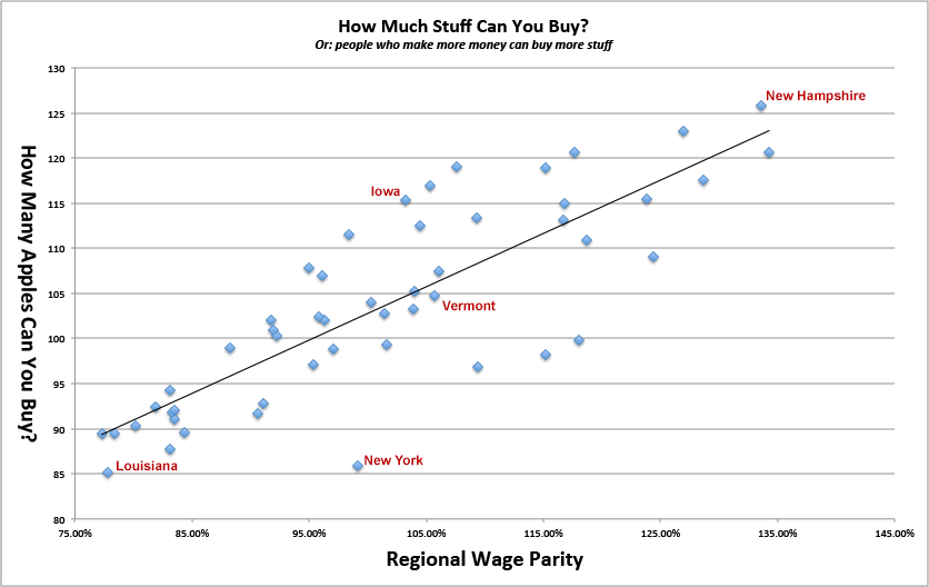
How many apples can you buy

Note, while local wages seem to predict well for this "how many apples" measure, prices do not seem to predict at all. Goes to show, cheap != affordable.
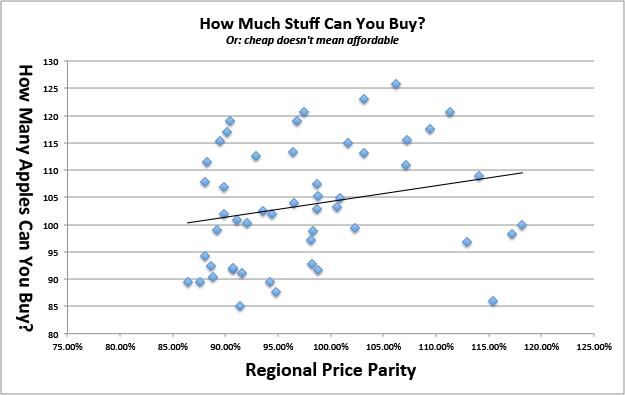
prices

Here's the raw data I used for this if you want to play around with it:

+----------------------+-----------------------+----------------------+------------------+
|        State         | Regional Price Parity | Regional Wage Parity | How Many Apples? |
+----------------------+-----------------------+----------------------+------------------+
| Louisiana            | 91.40%                | 77.81%               |               85 |
| New York             | 115.40%               | 99.14%               |               86 |
| New Mexico           | 94.80%                | 83.12%               |               88 |
| Mississippi          | 86.40%                | 77.30%               |               89 |
| Arkansas             | 87.60%                | 78.39%               |               89 |
| Montana              | 94.20%                | 84.35%               |               90 |
| Kentucky             | 88.80%                | 80.21%               |               90 |
| North Carolina       | 91.60%                | 83.45%               |               91 |
| Florida              | 98.80%                | 90.60%               |               92 |
| Tennessee            | 90.70%                | 83.27%               |               92 |
| South Carolina       | 90.70%                | 83.53%               |               92 |
| West Virginia        | 88.60%                | 81.89%               |               92 |
| Nevada               | 98.20%                | 91.10%               |               93 |
| Alabama              | 88.10%                | 83.07%               |               94 |
| California           | 112.90%               | 109.39%              |               97 |
| Arizona              | 98.10%                | 95.31%               |               97 |
| Hawaii               | 117.20%               | 115.16%              |               98 |
| Maine                | 98.30%                | 97.09%               |               99 |
| Ohio                 | 89.20%                | 88.24%               |               99 |
| Delaware             | 102.30%               | 101.61%              |               99 |
| District of Columbia | 118.20%               | 118.01%              |              100 |
| Georgia              | 92.00%                | 92.23%               |              100 |
| Indiana              | 91.10%                | 91.93%               |              101 |
| Michigan             | 94.40%                | 96.26%               |              102 |
| Oklahoma             | 89.90%                | 91.71%               |              102 |
| Idaho                | 93.60%                | 95.86%               |              102 |
| Pennsylvania         | 98.70%                | 101.48%              |              103 |
| Illinois             | 100.60%               | 103.93%              |              103 |
| Texas                | 96.50%                | 100.33%              |              104 |
| Vermont              | 100.90%               | 105.73%              |              105 |
| Oregon               | 98.80%                | 103.97%              |              105 |
| Kansas               | 89.90%                | 96.16%               |              107 |
| Rhode Island         | 98.70%                | 106.07%              |              107 |
| Missouri             | 88.10%                | 95.00%               |              108 |
| New Jersey           | 114.10%               | 124.36%              |              109 |
| Alaska               | 107.10%               | 118.71%              |              111 |
| South Dakota         | 88.20%                | 98.39%               |              112 |
| Wisconsin            | 92.90%                | 104.50%              |              112 |
| Washington           | 103.20%               | 116.72%              |              113 |
| Wyoming              | 96.40%                | 109.30%              |              113 |
| Colorado             | 101.60%               | 116.78%              |              115 |
| Iowa                 | 89.50%                | 103.26%              |              115 |
| Massachusetts        | 107.20%               | 123.79%              |              115 |
| Nebraska             | 90.10%                | 105.34%              |              117 |
| Connecticut          | 109.40%               | 128.66%              |              118 |
| Utah                 | 96.80%                | 115.15%              |              119 |
| North Dakota         | 90.40%                | 107.59%              |              119 |
| Minnesota            | 97.50%                | 117.62%              |              121 |
| Maryland             | 111.30%               | 134.28%              |              121 |
| Virginia             | 103.20%               | 126.95%              |              123 |
| New Hampshire        | 106.20%               | 133.56%              |              126 |
+----------------------+-----------------------+----------------------+------------------+

Sources:
Wage data (Direct XLS Download)
Price Data (PDF)

$\endgroup$
9
$\begingroup$

A bit dated, but here are Real Personal Income and Regional Price Parities for States and Metropolitan Areas, 2008–2012. The BEA takes per capita personal income by state and normalizes it by a cost of living index specific to that state.

They find that New York and California are about 13 percent (119/106) more expensive than the country as a whole in 2012. Nevertheless, the average real income per capita in those states is 39 in CA, 44 in NY, and 41 nationally, suggest that even though CA is richer before cost adjustment (1.19 * 39 > 41 * 1.06) the higher income does not afford a larger bundle of goods taking into account the higher cost of living. NY is both more expensive and richer. All numbers from Table 1 on page 7.

Note, however, P. J. O'Rourke's quip about cost of living adjustments:

PPP is supposed to compensate for the lower living costs found in poorer countries. It's like having your boss tell you , "Instead of a raise, why don't you move to a worse neighborhood -- your rent will be lower and so will your car payments, as soon as someone steals your Acura."

That is, the cost of living reflects the prices of living and some of the differences in those prices reflect demand differences related to amenities which are not typically captured in these costs of living. For example, a safe neighborhood may be more expensive than an unsafe one and that safety the reason for the price differences between neighborhoods. Correcting for price differences captures the differences in house prices but over-corrects because at the same prices families prefer the safe neighborhood. This problem exists for almost all amenities; parks, Broadway, the Smithsonian, and school quality to name a few. In fact, virtually the only feature of housing that does not suffer from this problem (in theory anyway) is the access to good jobs because the capitalized value of access to high paying jobs is exactly the income from those higher paying jobs that accrues to the current land owners and not workers and so should be rightly subtracted from wages when comparing wages in two regions.

$\endgroup$
2
  • $\begingroup$ Thank you for your thoughtful reply. Your point is well taken, I see that this is indeed a topic of some complexity. You'll forgive me, but I'm not sure I have the appropriate training to interpret the data in the article you linked. Could you help translate the findings for a lay person? $\endgroup$ Commented Mar 3, 2015 at 0:45
  • $\begingroup$ Thanks again for the helpful edit to this question. I would upvote you if I could, but I don't have enough reputation. $\endgroup$ Commented Mar 3, 2015 at 4:29
0
$\begingroup$

Many events/services/products exists in NY but not in Louisiana. This increased variety and possibilities is more qualitative. It depends on the "utility" derived for this increased cultural/commercial avtivities. But there is a large offer of music events a NewYorker can easily attend after the job, while a person living in a less densily populated area would have to take a flight. Large urban centers offers certain agglomerative benefits that are underestimated when comparing identical basket of goods. Also, in NY you may not need a car a probably live in a smaller appartment than you would otherwise. So a for city-dweller his utility can offset living costs but the nature-lover is probably much worse off (especially considering congestion on friday pm.) The concept of Utility cannot be measured precisely but helps to explain why people choose sunny California even if they are worse off "financially".

$\endgroup$

Your Answer

By clicking “Post Your Answer”, you agree to our terms of service and acknowledge you have read our privacy policy.

Not the answer you're looking for? Browse other questions tagged or ask your own question.