Question
I want to compute the Bayesian equilibria for the following Bayesian game:
 With probability $p$, player 1 would be of type 1.1. With probability $1-p$, player 1 would be of type 1.2. Player 2 does not have any private information and she only has one type 2.0.
I know two methods to compute Bayesian equilibria. The first one, with which I think I am more familiar, is based on the presentation from Roger Myerson's Game Theory: Analysis of conflict. The other one is presented by William Spaniel's Game Theory 101 Youtube course. I want to use both method to solve this question and, of course, I expect to get the same result. But I got some trouble when proceeding William Spaniel's method. I would really appreciate it if someone could help me figure out where my problem is!
Method 1$\quad$[Roger Myerson]
This is the same answer I worte for this MSE post. But I will present it here as well.
Note that a Bayesian equilibrium of the game $\Gamma^b$ is any randomized-strategy profile $\sigma$ such that, for every player $i$ in $N$ and every type $t_i$ in $T_i$, \begin{align*} \sigma_i(\cdot|t_i) \in \text{argmax}_{\tau_i \in \Delta(C_i)} \sum_{t_{-i} \in T_{-i}} p_i(t_{-i}|t_i) \sum_{c\in C}\left(\prod_{j \in N-i}\sigma_j(c_j|t_j)\right)\tau_i(c_i)u_i(c,t). \end{align*} As for our game, we make the following definition:
$C_1 = \{x_1,y_1\}$, where $x_1$ means "up" and $y_1$ means "down".
$C_2 = \{x_2,y_2\}$, where $x_2$ means "left" and $y_2$ means "right".
$C = C_1\mathop{\Large\times}C_2$
$\Delta(C)$ is the set of all probability distributions over the set $C$
$T_1 = \{1.1,1.2\}$, where 1.1 stands for player 1's type of coorperative and 1.2 stands for player 1's type of uncooperative.
$T_2 = \{2.0\}$, where 2.0 stands for player 2's only possible type.
$T = T_1\mathop{\Large\times}T_2$
$p_2(1.1|2.0) = p$ and $p_2(1.2|2.0) = 1-p$, where $p_2(\cdot|2.0)$ represents what player 2 would believe about player 1's types given his own type being 2.0.
First, consider the matrix for $t_1=1.1$. Clearly, there are two pure strategy Nash equilibria: \begin{align*} \sigma_1(\cdot|1.1)=[x_1],\ \sigma_2=[x_2]\quad \text{and}\quad \sigma_1(\cdot|1.1)=[y_1],\ \sigma_2=[y_2], \end{align*} and one mixed strategy Nash equilibrium: \begin{align*} \sigma_1(\cdot|1.1)=\frac{1}{2}[x_1]+\frac{1}{2}[y_1],\ \sigma_2 = \frac{1}{2}[x_2] + \frac{1}{2}[y_2]. \end{align*}
Next, consider the matrix for $t_1 = 1.2$. Clearly, there is only one Nash equilibrium: \begin{align*} \sigma_1(\cdot|1.2)=\frac{1}{2}[x_1]+\frac{1}{2}[y_1],\ \sigma_2 = \frac{1}{2}[x_2] + \frac{1}{2}[y_2]. \end{align*}
Therefore, we have the following three cases:
Case 1:$\quad$[Mixed strategy Nash equilibria for both matrices]
Since \begin{align*} \begin{alignedat}{4} &p_2(1.1|2.0) \cdot (&&\sigma_1(x_1|1.1) \cdot \tau_2(x_2) \cdot u_1((x_1,x_2),(1.1,2.0)) &\ +\\ & &&\sigma_1(y_1|1.1) \cdot \tau_2(x_2) \cdot u_1((y_1,x_2),(1.1,2.0)) &\ +\\ & &&\sigma_1(x_1|1.1) \cdot \tau_2(y_2) \cdot u_1((x_1,y_2),(1.1,2.0)) &\ +\\ & &&\sigma_1(y_1|1.1) \cdot \tau_2(y_2) \cdot u_1((y_1,y_2),(1.1,2.0)))&\\ =\ &0 && & \end{alignedat} \end{align*} and \begin{align*} \begin{alignedat}{4} &p_2(1.2|2.0) \cdot (&&\sigma_1(x_1|1.2) \cdot \tau_2(x_2) \cdot u_1((x_1,x_2),(1.2,2.0)) &\ +\\ & &&\sigma_1(y_1|1.2) \cdot \tau_2(x_2) \cdot u_1((y_1,x_2),(1.2,2.0)) &\ +\\ & &&\sigma_1(x_1|1.2) \cdot \tau_2(y_2) \cdot u_1((x_1,y_2),(1.2,2.0)) &\ +\\ & &&\sigma_1(y_1|1.2) \cdot \tau_2(y_2) \cdot u_1((y_1,y_2),(1.2,2.0)))&\\ =\ &0, && & \end{alignedat} \end{align*} it follows that \begin{align*} &\text{argmax}_{\tau_2 \in \Delta(C_2)} \sum_{t_{1} \in T_{1}} p_2(t_{1}|t_2) \sum_{c\in C}\left(\prod_{j \in \{1\}}\sigma_j(c_j|t_j)\right)\tau_2(c_2)u_2(c,t)\\ =\ &\text{argmax}_{\tau_2 \in \Delta(C_2)} 0\\ =\ &0. \end{align*} Thus, $\sigma_2(\cdot|2.0) = \alpha[x_2] + (1-\alpha)[y_2]$ for all $\alpha \in [0,1]$, $\sigma_1(\cdot|1.1) = \frac{1}{2}[x_1]+\frac{1}{2}[y_1]$, and $\sigma_1(\cdot|1.2) = \frac{1}{2}[x_1] + \frac{1}{2}[y_1]$ is a Bayesian equilibrium.
Case 2:$\quad$[The first pure equilibrium for matrix $\mathbf{t_1=}\ $1.1]
Since \begin{align*} p_2(1.1|2.0)\cdot(1\cdot\tau_2(x_2)\cdot1+0+1\cdot\tau_2(y_2)\cdot(-1)+0) = p(\tau_2(x_2)-\tau_2(y_2)), \end{align*} it follows that \begin{align*} &\text{argmax}_{\tau_2 \in \Delta(C_2)} \sum_{t_{1} \in T_{1}} p_2(t_{1}|t_2) \sum_{c\in C}\left(\prod_{j \in \{1\}}\sigma_j(c_j|t_j)\right)\tau_2(c_2)u_2(c,t)\\ =\ &\text{argmax}_{\tau_2 \in \Delta(C_2)} p\cdot(\tau_2(x_2)-\tau_2(y_2))\\ =\ &(\tau_2(x_2)=1,\tau_2(y_2)=0)\\ =\ &[x_2]. \end{align*} Thus, $\sigma_2(\cdot|2.0)=[x_2]$, $\sigma_1(\cdot|1.1)=[x_1]$, and $\sigma_1(\cdot|1.2) = \frac{1}{2}[x_1]+\frac{1}{2}[y_1]$ is a Bayesian equilibrium.
Case 3:$\quad$[The second pure equilibrium for matrix $\mathbf{t_1=}\ $1.1]
Since \begin{align*} p_2(1.1|2.0)\cdot(0+1\cdot\tau_2(x_2)\cdot(-1)+0+1\cdot\tau_2(y_2)\cdot1) = p(\tau_2(y_2)-\tau_2(x_2)), \end{align*} it follows that \begin{align*} &\text{argmax}_{\tau_2 \in \Delta(C_2)} \sum_{t_{1} \in T_{1}} p_2(t_{1}|t_2) \sum_{c\in C}\left(\prod_{j \in \{1\}}\sigma_j(c_j|t_j)\right)\tau_2(c_2)u_2(c,t)\\ =\ &\text{argmax}_{\tau_2 \in \Delta(C_2)} p\cdot(\tau_2(y_2)-\tau_2(x_2))\\ =\ &(\tau_2(x_2)=0,\tau_2(y_2)=1)\\ =\ &[y_2]. \end{align*} Thus, $\sigma_2(\cdot|2.0)=[y_2]$, $\sigma_1(\cdot|1.1)=[y_1]$, and $\sigma_1(\cdot|1.2) = \frac{1}{2}[x_1]+\frac{1}{2}[y_1]$ is a Bayesian equilibrium.
Method 2$\quad$ [William Spaniel]
You may refer to this short video for his presentation. The idea of this method is to transfer the original type-agent representation to an "averaged" game matrix, and find the Nash equilibria for the new matrix.
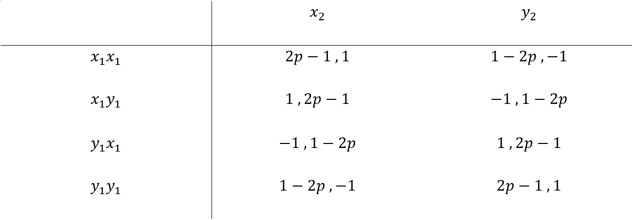
The new "averaged" game matrix I got is the following:
 But how should I proceed next? What bothers me is the variable $p$. For example, when $p=1$, then there are four pure strategy Nash equilibria: $(x_1x_1,x_2), (x_1y_1,x_2), (y_1x_1,y_2), (y_1y_1,y_2)$. But I don't think any of the Bayesian equilibria computed in Method 1 is compatible with them. I am baffled.
My Problem
It might be that my Method 1 has some problems (I'm not sure). But I just didn't think I can get the same result using the two methods. And I don't know what to do with method 2. Could someone please help me out?
Related Definition from Myerson's Text
Definition of A Bayesian Game$\quad$ To define a Bayesian game (or a game in Bayesian form), we must specify a set of players $N$ and, for each player $i$ in $N$, we must specify a set of possible actions $C_i$, a set of possible types $T_i$, a probability function $p_i$, and a utility function $u_i$. We let \begin{align*} C = \mathop{\Large\times}_{i \in N} C_i,\quad T = \mathop{\Large\times}_{i \in N} T_i. \end{align*} That is, $C$ is the set of all possible profiles or combinations of actions that the players may use in the game, and $T$ is the set of all possible profiles or combinations of types that the player may have in the game. For each player $i$, we let $T_{-i}$ denote the set of all possible combinations of types for the players other than $i$, that is, \begin{align*} T_{-i} = \mathop{\Large\times}_{j \in N-i} T_j, \end{align*}
The probability function $p_i$ in the Bayesian game must be a function from $T_i$ into $\Delta(T_{-i})$, the set of probability distributions over $T_{-i}$. That is, for any possible type $t_i$ in $T_i$, the probability function must specify a probability distribution $p(\cdot|t_i)$ over the set $T_{-i}$, representing what player $i$ would believe about the other players' types if his own type were $t_i$. Thus, for any $t_{-i}$ in $T_{-i}$, $p_i(t_{-i}|t_i)$ denotes the subjective probability that $i$ would assign to the event that $t_{-i}$ is the actual profile of types for the other players, if his own type were $t_i$.
For any player $i$ in $N$, the utility function $u_i$ in the Bayesian game must be a function from $C \times T$ into the real numbers $\mathbb{R}$. That is, for any profile of actions and types $(c,t)$ in $C \times T$, the function $u_i$ must specify a number $u_i(c,t)$ that represents the payoff that player $i$ would get, in some von Neumann-Morgenstern utility scale, if the players' actual types were all as in $t$ and the players all chose their actions as specified in $c$.
These structures together define a Bayesian game $\Gamma^b$, so we may write \begin{equation} \Gamma^b = \left(N, (C_i)_{i \in N}, (T_i)_{i \in N}, (u_i)_{i \in N}\right). \end{equation} $\Gamma^b$ is finite if and only if the sets $N$ and $C_i$ and $T_i$ (for every $i$) are all finite.
Definition of Bayesian Nash Equilibrium$\quad$ To formally state the definition of a Bayesian equilibrium, let $\Gamma^b$ be a Bayesian game, so \begin{align*} \Gamma^b = (N, (C_i)_{i \in N}, (T_i)_{i \in N}, (p_i)_{i \in N}, (u_i)_{i \in N}). \end{align*} A randomized-strategy profile for the Bayesian game $\Gamma^b$ is any $\sigma$ in the set $\mathop{\Large\times}_{i \in N} \mathop{\Large\times}_{t_i \in T_i} \Delta(C_i)$, that is, any $\sigma$ such that \begin{align*} &\sigma = \left((\sigma_i(c_i|t_i))_{c_i \in C_i}\right)_{t_i \in T_i,i \in N},\\ \\ &\sigma_i(c_i|t_i) \geq 0,\quad \forall c_i \in C_i,\quad \forall t_i \in T_i,\quad \forall i \in N,\quad \text{and}\\ \\ &\sum_{c_i \in C_i} \sigma_i(c_i|t_i) = 1,\quad \forall t_i \in T_i,\quad \forall i \in N. \end{align*} In such a randomized-strategy profile $\sigma$, the number $\sigma_i(c_i|t_i)$ represents the conditional probability that player $i$ would use action $c_i$ if his type were $t_i$. In the randomized-strategy profile $\sigma$, the randomized strategy for type $t_i$ of player $i$ is \begin{align*} \sigma_i(\cdot|t_i) = (\sigma_i(c_i|t_i))_{c_i \in C_i}. \end{align*} A Bayesian equilibrium of the game $\Gamma^b$ is any randomized-strategy profile $\sigma$ such that, for every player $i$ in $N$ and every type $t_i$ in $T_i$,
An Example from William Spaniel's Lecture
Here is the game matrix he presented in his lecture:
 With probability $0.2$, player 2 would be of type 2.1. With probability $0.8$, player 2 would be of type 2.2.
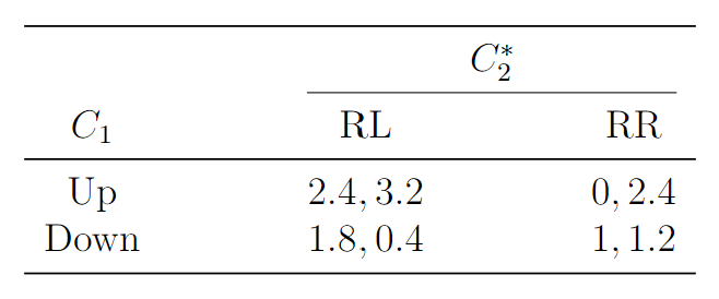
In order to compute the Bayesian equilibria, William converted the original type-agent representation into a "weighted-averaged" game matrix. We got rid of the different types of player 2 and combined them into just a single player. So we have the following four columns: $LL$, $LR$, $RL$, $LL$. The interpretation is, for example, the $LL$ column stands for both type 2.1 and type 2.2 are going to choose "Left"; the $LR$ column stand for just type 2.1 is going to choose "Left" and just type 2.2 is going to choose "Right". In order to fill in the payoff matrix, we calculate the expected payoff for each player in each cell, and we will get the following matrix:
 Notice that the first column is strongly dominated by the third column, and that the second column is strongly dominated by the fourth column. So, we can reduce this $2\times 4$ matrix to the following $2 \times 2$ matrix:
 Compute the Nash equilibrium for it, we have
- $(\text{[Up]}, \text{[RL]})$
- $(\text{[Down]}, \text{[RR]})$, and
- $(\frac{1}{2}\text{[Up]}+\frac{1}{2}\text{[down]}, \frac{5}{8}\text{[RL]}+\frac{3}{8}\text{[RR]})$.
The interpretation of the three Bayesian Nash equilibria is the following, respectively:
- There is a Bayesian Nash equilibrium in which player 1 chooses "$\text{Up}$", player 2 as type 2.1 chooses "$\text{Right}$", and player 2 as type 2.2 chooses "$\text{Left}$".
- There is a Bayesian Nash equilibrium in which player 1 chooses "$\text{Down}$" and player 2 as both type 2.1 and 2.2 choose "$\text{Right}$".
- There is a mixed strategy Bayesian Nash equilibrium in which player 1 chooses "$\text{Up}$" with probability $\frac{1}{2}$ and "$\text{Down}$" with probability $\frac{1}{2}$, player 2 as type 2.1 chooses "$\text{Right}$" with probability $1$ (because $\frac{5}{8}+\frac{3}{8}=1$), and player 2 as type 2.2 chooses "$\text{Left}$" with probability $\frac{5}{8}$ and "$\text{Right}$" with probability $\frac{3}{8}$.
Please help! Pretty Please! Thank you very much!
