I was experimenting with a seemingly simple optimal control problem that generates a system of differential equations. When I calculate the values of the steady state of the system I get some very strange results I believe I did something wrong when I applied the Maximum Principle. If you are patient enough to read some text, I would be grateful to listen to your suggestions what could go wrong.
Notation
I use a subscript $t$ whenever a variable depends on time. E.g. $A_t(x_1,x_2):=A(x_1,x_2,t)$
Setup
Imagine a closed-economy with a linear production function. The amount of goods produced depends on the level of human capital $A_t$ and some fixed ressource endowment $R$. Thus,
$Y_t := A_tR$
The economy we imagine has an insecure environment and can be attacked at random with a probability of $p$ (exogenous). Whenever country is attacked, it losses some of its income. I denote the remaining share $q_t$. The share of income protected depends on the amount of military spending the country has augmented by the level of human capital accumulated:
$q_t:=1-\frac{1}{\alpha A^m_t M_t}$
I assume $m \in [0,1]$ Thus the greater is military spending, the more secure is current income. Note that military spending does better job in securing protection as long as $m<1$.
Given all this, assume the economy produces 3 types of goods: consumption goods $C_t$, military goods $M_t$ and human capital $A_t$. Assume for simplicity, that $A_t$ is the only variable that accumulates while consumption goods and military goods are consumed instantaneously at every moment in time. If one agrees on this, one way of expressing the equation of motion for human capital is the weighted average of income the country has minus spending on consumption, military and deprecitation of human capital:
$\dot{A}_t=\underbrace{pq_tY_t}_\text{Post-war income} + \underbrace{(1-p)Y_t}_\text{No-war income} - C_t - M_t - \delta A_t$
Assuming that all variables belong to the positive real line, additionaly $A_t,M_t>0$, a concave utility function $U'(C_t)>0, U''(C_t)<0$ and `granting' some initial value of human capital $A(t=0)=A_0$ one can formulate the following optimal control problem: \begin{equation} \max_{C_t, M_t}\int_0^\infty U(C_t)e^{-\rho t}dt \end{equation}
In words: maximize utility over infinite horizon steering consumption and military.
Such that: \begin{equation} \dot{A}_t=p\left(1-\frac{1}{\alpha A^m_t M_t}\right)A_tR + (1-p)A_tR - C_t - M_t - \delta A_t \end{equation} And the transversality condition: \begin{equation} \lim_{t->\infty} e^{-\rho t}\lambda_t A_t=0 \end{equation}
Hamiltonian and Solution
The current-value Hamiltonian looks like this ($\mu_t = \lambda_t e^{-\rho t}$): \begin{equation} H^c = U(C_t) + \mu_t\left(p\left(1-\frac{1}{\alpha A^m_t M_t}\right)A_tR + (1-p)A_tR - C_t - M_t - \delta A_t\right) \end{equation}
Chiang (1992) argues that if the Hamiltonian is nonlinear in control and state variables, one derive the first-order conditions by taking derivatives of the Hamiltonian and setting them equal to zero.
\begin{equation} \frac{\partial H^c}{\partial C_t}: U'(C_t)-\mu_t = 0 \end{equation}
\begin{equation} \frac{\partial H^c}{\partial C_t}: \mu_t\left(pA^{1-m}_tR\frac{1}{\alpha M^2_t}-1\right) = 0 \end{equation}
\begin{equation} \dot{\mu}_t = \rho \mu_t - \mu_t\left(pR\frac{m-1}{\alpha A^m_t M_t} + R - \delta\right) \end{equation}
The expressions for $\dot{\mu}_t$ and $\dot{A}_t$ form a system of differential equations. But interpreting \dot{\mu}_t is counter-intuitive. Instead, one usually differentiates the FOC for consumption with respect to time $U''(C)_t=\dot{\mu}_t$ and impute \dot{\mu}_t from the equation of motion. Since $U'(C_t) = \mu_t$, one can get rid of $\mu_t$ in $\dot{C}_t$. Yet, the system will consist of two equations $\dot{C}_t, \dot{A}_t$ and three variables $A_t$, $C_t$, $M_t$.
\begin{equation} \begin{cases} \dot{C}_t = -\frac{U'(C_t)}{U''(C_t)}\left(pR\frac{m-1}{\alpha A^m_t M_t} + R - \delta -\rho\right) \\ \dot{A}_t = A_t R - A^{1-m}_t\frac{pR}{M_t} - C_t - M_t - \delta A_t \end{cases} \end{equation}
I need a way to express $M_t$ as a function of other variables or parameters. Thus I take the second FOC, equate it to zero (dismiss the option $\mu_t=0$ because $\mu_t=U'(C_t)>0$) and derive $M_t$ as a function of $A_t$: $M^*_t:=A^{\frac{1-m}{2}}_t\sqrt{\frac{pR}{\alpha}}$
I impute $M^*_t$ in the system above, set $\dot{C}_t=\dot{A}_t=0$ and calculate the expressions for the steady state. Dismissing the trivial solution $C_t = 0$, I obtain the following equilibrium values:
Human Capital
\begin{equation} \bar{A}_t = \left(\frac{pR}{\alpha}\frac{(1-m)^2}{(R - \delta -\rho)^2}\right)^{\frac{1}{1+m}} \end{equation}
Military
\begin{equation} \bar{M_t} = \left(\frac{pR}{\alpha}\frac{(1-m)^2}{(R - \delta -\rho)^2}\right)^{\frac{1-m}{2(1+m)}}\sqrt{\frac{p R}{\alpha}} \end{equation}
Consumption
\begin{multline} \bar{C_t} = \left(\frac{pR}{\alpha}\frac{(1-m)^2}{(R - \delta -\rho)^2}\right)^{\frac{1}{1+m}} (R - \delta) \\- \left(\frac{pR}{\alpha}\frac{(1-m)^2}{(R - \delta -\rho)^2}\right)^{\frac{1-m}{2(1+m)}} \sqrt{\alpha pR} \left(1 + \frac{1}{\alpha}\right) \end{multline}
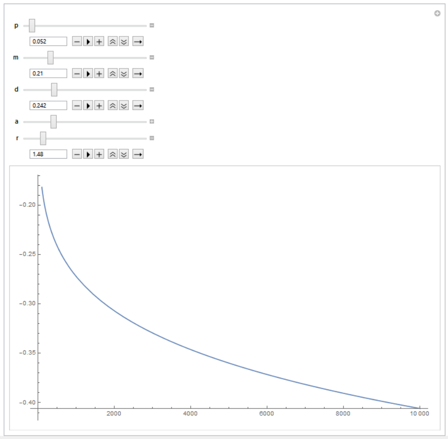
The expression for consumption looks clumsy. It is indeed! When I tried to calculate values of consumption given some more or less reasonable parameters ($p=0.052$, $m=0.21$, $\delta=0.242$, $\alpha = 2.54$, $\rho=1.48$), I got negative numbers. A screenshot from Mathematica depicting $C_t$ (vertical axis) as a function of $R$ (horizontal axis):
I do not expect that introducing insecure property rights will change the steady state consumption to negative values given a linear production function. It looks that I applied the Maximum Principle algorithm in a wrong way but I cannot figure out what was my mistake. Could somebody point me what went wrong? Any ideas? P.S. You are a hero if you read till the very end :)
UPDATE: As some of people here suggested, the Maximum Principle fails because I apply deterministic method to a stochastic model. This is a fair concern. I decided to check if the method works in case I set $p=1$ (implying the infinitely long war-scenario for the economy).
The canonical equations with the specification look like that:
\begin{equation} \frac{\partial H^c}{\partial C_t}: U'(C_t)-\mu_t = 0 \end{equation}
\begin{equation} \frac{\partial H^c}{\partial C_t}: \mu_t\left(pA^{1-m}_tR\frac{1}{\alpha M^2_t}-1\right) = 0 \end{equation}
\begin{equation} \dot{\mu}_t = \rho \mu_t - \mu_t\left(R - R\frac{1-m}{\alpha A^m_t M_t} - \delta\right) \end{equation}
I proceeded with the solution as before and got the following dynamical system (assuming $U(C_t)=\ln{C_t}$:
\begin{equation} \begin{cases} \dot{C}_t = C_t\left(R - R\frac{1-m}{\alpha A^m_t M_t} + R - \delta -\rho\right) \\ \dot{A}_t = A_t R - A^{1-m}_t\frac{R}{M_t} - C_t - M_t - \delta A_t \end{cases} \end{equation}
Solve it for the steady state. Here are my equilibrium values for Human Capital, Military and Consumption.
\begin{equation} \bar{A}=\left(\frac{(1-m)^2}{(R-\delta-\rho)^2} \frac{R}{\alpha} \right)^{\frac{1}{1+m}} \end{equation}
\begin{equation} \bar{M}=\left(\frac{R}{\alpha}\right)^{1/2}\left(\frac{(1-m)^2}{(R-\delta-\rho)^2} \frac{R}{\alpha} \right)^{\frac{1-m}{2(1+m)}} \end{equation}
\begin{equation} \bar{C}=(R-\delta)\left(\frac{(1-m)^2}{(R-\delta-\rho)^2} \frac{R}{\alpha} \right)^{\frac{1}{1+m}}-2\left(\frac{R}{\alpha}\right)^{1/2}\left(\frac{(1-m)^2}{(R-\delta-\rho)^2} \frac{R}{\alpha}\right)^{\frac{1-m}{2(1+m)}} \end{equation}
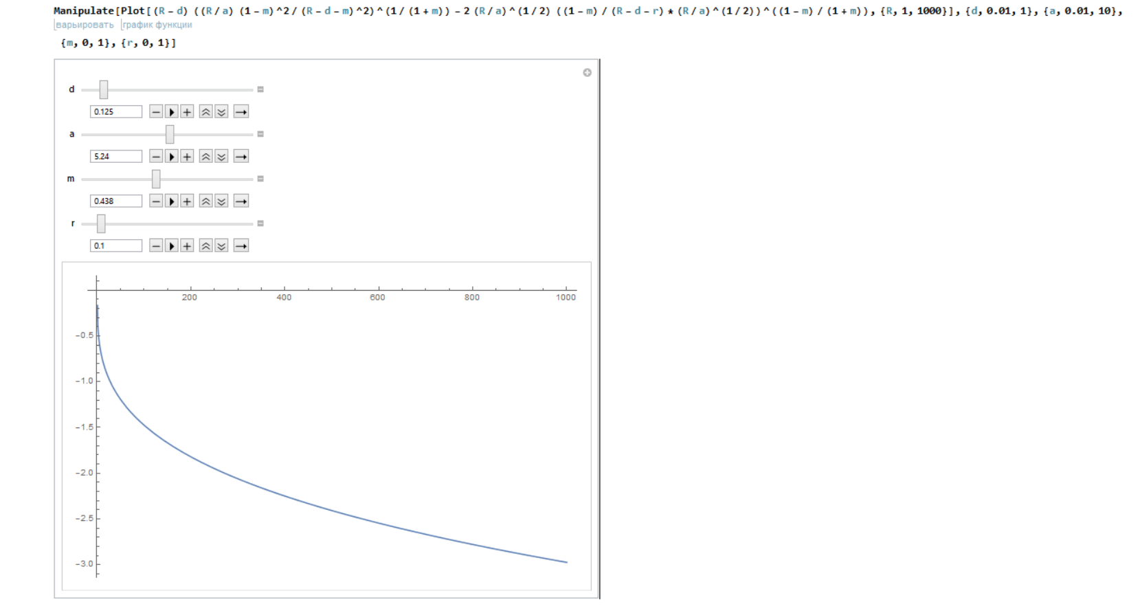
I simulated the values of $C_t$ again. Here is what I get:

Different equations, yet similar picture. So the stochastic nature of the model is not the only problem. Maybe I miss something like a bang-bang solution here? Or maybe it simply does not exist in the case?