GE with an intermediate good

Question

intro

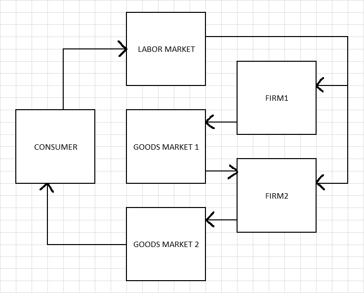
I'm looking at a simple model with 1 consumer, 2 goods and 2 firms.

I'm trying to get a price vector [p0, p1] that makes it work.

By makes it work, I mean, supply = demand in all 3 markets.

the problem

The problem is that I'm actually getting a set of price vectors that work.

Consider the picture below :

little details

consumer

There is one consumer who owns both firms and their profits and they go :

$$ u = \ln x + \gamma \ln b $$ where $b$ is leisure, and $\gamma$ is their relative want of leisure

And their budget is :

$$ M = wL + \pi_0+ \pi_1 $$ where $w$ is wage, $L$ is their time endowment ($n + b = L$), and $\pi_0$ and $\pi_1$ are each firm's profits.

Solving that gives $x$ and $b$, so labor supply is $n = L - b$.

$$b=\dfrac{\gamma}{1+\gamma} \cdot \dfrac{M}{w}, 0 < b < L$$ $$x=\dfrac{1}{1+\gamma} \cdot \dfrac{M}{p_1}$$ $$n=L-b$$

firms[0]

The first firm, firms[0], uses just labor to make an intermediate good :

$$\pi_0 = p_0 \cdot z_0^{\alpha} - w z_0$$ where $0 < \alpha < 1$, $z_0$ is their labor demand, and $y_0 = z_0^{\alpha}$ is their output.

firms[1]

The other firm, firms[1], uses labor and firms[0]'s output, $y_0$.

$$\pi_1 = p_1 \cdot z_1^{\beta} \cdot (k_1+1)^{1-\beta} - w \cdot z_1 - p_0 \cdot k_1$$

Here, $z_1$ is their labor demand, $k_1$ is their intermediate goods demand, and $0 < \beta < 1$. Their output is $y_1=f_1(z_1,k_1)=z_1^{\beta} \cdot (k_1+1)^{1-\beta}$

This firm is almost constant returns to scale. That is, if it can make profit at some level $(z_1,k_1)$, then it will make more profit at $(az_1,ak_1)$ where $a>1$. That means that this firm won't settle on some profit maximizing allocation of $(z_1,k_1)$ since it will choose to keep buying more, at a given price level. So this firm uses $y_0$ as its limiting factor. And from there it decides how much labor to use.

Also, I made it so that $k_1$ could be 0. So like, depending on $[\alpha, \beta, \gamma, L]$ it could be that firms[0] doesn't even produce.

the markets

So the markets look like this :

Labor : n = z[0] + z[1] @ w

Middle : y[0] = k[1] @ p[0]

Final : y[1] = x @ p[1]

how i'm solving them

First, it's important to note that I do not know what I am doing. I'm doing this purely out of boredom, so please don't be surprised if the answer is something really obvious and I just plum don't know about it.

So I have a little function that takes some random price, say [1, 1], and uses that price vector to get the sum of squares of excess supply, exx. Like, it does "supply minus demand" for each market and squares it, and adds it to the total. It's my way of measuring how bad a price vector is. (Is there a way to measure how bad a price vector is?)

Then it checks a bunch of price vectors around it, like [1+dp, 1], [1-dp, 1], [1, 1+dp] etc.. where dp is the size of the step. And when finds a point around it with a lower exx, it makes that the new price. And repeats. And when it doesn't find a better point, it shrinks dp and does it again.

the problem

The price vector I get changes depending on the starting point. And most of the time I get an exx = 0 (or very very near 0). The problem is that (just based on my graphing it), exx(p[0],p[1]) doesn't seem to be continuous. When I graph exx against p[0] (x-axis) and p[1] (y-axis), I get a whole set (a line) of price vectors and when I check them manually, they work.

centrally planned

When I solve the central planner problem it looks like this :

$$u= \ln x + \gamma \cdot \ln b$$

But $x=y_1=z_1^{\beta} \cdot (k_1+1)^{1-\beta}$ and $k_1=y_0=z_0^{\alpha}$ so that gives the following :

$$u = \beta \cdot \ln n_1 + (1-\beta) \cdot \ln (n_0^{\alpha} + 1) + \gamma \cdot \ln (L - n_0 - n_1)$$

Take $\frac{du}{dn_0}$ and $\frac{du}{dn_1}$ and that gives you something like :

$$0 = C_0 \cdot n_0^{1-\alpha} + C_1 \cdot n_0 + C_2$$

Where $[C_0, C_1, C_2]$ are constants made from the the exogenous variables $[\alpha, \beta, \gamma, L]$

Which is an equation I don't know how to solve but I do it numerically and I can verify that it is the utility-maximizing allocation.

I guess for me the important thing is the solution this gives is on that line I get when I graph $exx$ against $p_0$ and $p_1$. Important insofar as the algorithmic approach I used isn't too wrong, that is.

Anyhow, the reason I want the algorithmic approach to work is because I can easily add lots of consumers, firms, products, firm ownerships etc, and in order to do that, which is fun, I need to make sure my approach, in a technical sense, is sound and actually works.

questions

Does this problem have a unique solution?

Is there a proper way of solving for the solution(s)?

I guess that's all. I can possibly add a link to the work I did.

edit: 2021-06-22

Here's a link to where I'm playing around with this. There seem to be lots of price vectors that work. But since I'm solving them numerically, 'work' really just means 'below a certain level of error'.

https://dactyrafficle.github.io/GE_intermediate/

Answer 1

This is my attempt. The final result is a set of equilibrium equations, which I will not attempt at solving.

The consumer:

$$ \max \ln(x) + \gamma \ln(b) \text{ s.t. } p_1 x + w b = w L + \pi_0 + \pi_1. $$

This is Cobb-Douglass so: $$ \begin{align*} &x_1 = \frac{1}{1 + \gamma} \frac{(wL + \pi_0 + \pi_1)}{p_1},\tag{1}\\ &b = \frac{\gamma}{1 + \gamma} \frac{(wL + \pi_0 + \pi_1)}{w}.\tag{2} \end{align*} $$

Firm 0

Firm 1 maxmizes $$ \pi_0 = p_0 z_0^\alpha - w z_0. $$ First order condition is: $$ \begin{align*} &p_0 \alpha z_0^{\alpha - 1} = w,\\ \to &z_0 = \left(\frac{w}{\alpha p_0}\right)^{1/(\alpha-1)},\tag{3}\\ \to &y_0 = \left(\frac{w}{\alpha p_0}\right)^{\alpha/(\alpha-1)},\tag{4}\\ \end{align*} $$ Profits are: $$ \pi_0 = p_0 \left(\frac{w}{\alpha p_0}\right)^{\alpha/(\alpha-1)} - w\left(\frac{w}{\alpha p_0}\right)^{1/(\alpha-1)}. \tag{5} $$

Firm 1

The first order conditions for profit maximisation of firm 1 give: $$ \beta \frac{y_1}{z_1} = \frac{w}{p_1},\\ (1-\beta) \frac{y_1}{(k_1 + 1)} = \frac{p_0}{p_1}. $$ taking ratios gives: $$ \frac{\beta (k_1 + 1)}{(1-\beta)z_1} = \frac{w}{p_0} $$ Now let's substitute this back into the production function: $$ \begin{align*} y_1 &= z_1^\beta (k_1 + 1)^{1-\beta},\\ &= \left(\frac{\beta}{1-\beta}\frac{p_0}{w} (k_1 + 1)\right)^{\beta}(k_1 + 1)^{1-\beta},\\ &= (k_1 + 1) \left(\frac{\beta}{1-\beta}\frac{p_0}{w}\right)^{\beta} \tag{6} \end{align*} $$ Also substituting $(k_1 + 1)$ instead gives: $$ y_1 = z_1^\beta \left(\frac{1-\beta}{\beta}\frac{w}{p_0}z_1\right)^{1-\beta},\\ = z_1 \left(\frac{1- \beta}{\beta} \frac{w}{p_0}\right)^{1-\beta} \tag{7} $$ Let's use these two expressions to compute the cost function: $$ w z_1 + p_0 k_1 = w y_1\left(\frac{1-\beta}{\beta}\frac{w}{p_0}\right)^{1/(1-\beta)} + p_0 y_1 \left(\frac{\beta}{1 - \beta}\frac{p_0}{w}\right)^{1/\beta} - p_0 $$ Notice the $-p_0$ at the end. So the profit is given by: $$ p_1 y - y_1\left(w \left(\frac{1 - \beta}{\beta} \frac{w}{p_0}\right)^{1/(1-\beta} + p_0 \left(\frac{\beta}{1-\beta} \frac{p_0}{w}\right)^{1/\beta}\right) + p_0 $$

There is a linear term in $y_1$. If the coefficient of this term is strictly positive, then the firm will set $y_1 = \infty$. If the term is negative then $y_1 = 0$, but this corresponds to an amount $k_1 = -1$, which is impossible. So the only choice is where the term in front of $y_1$ is zero. This gives: $$ p_1 = \left(w \left(\frac{1 - \beta}{\beta} \frac{w}{p_0}\right)^{1/(1-\beta} + p_0 \left(\frac{\beta}{1-\beta} \frac{p_0}{w}\right)^{1/\beta}\right) \tag{8} $$ Then profits of firm 1 are given by $$ \pi_1 = p_0 \tag{9} $$

Equilibrium

On the final goods market, we must have that using $(1)$: $$ \begin{align*} &x = y_1,\\ \to&\frac{1}{1 + \gamma} \frac{(wL + \pi_0 + \pi_1)}{p_1} = y_1 \tag{eq-1} \end{align*} $$ On the intermediate goods market, we have using $(4)$ and $(6)$: $$ \begin{align*} &y_0 = k_1,\\ \to &\left(\frac{w}{\alpha p_0}\right)^{\alpha/(\alpha-1)} = y_1 \left(\frac{\beta}{1-\beta}\frac{p_0}{w}\right)^{1/\beta}-1 \tag{eq-2} \end{align*} $$ On the labour market we have using $(2)$, $(3)$ and $(7)$: $$ \begin{align*} &L - b = z_0 + z_1,\\ \to &L - \frac{\gamma}{1 + \gamma} \frac{(wL + \pi_0 + \pi_1)}{w} = y_1\left(\frac{1- \beta}{\beta} \frac{w}{p_0}\right)^{1/(1-\beta)} + \left(\frac{w}{\alpha p_0}\right)^{1/(\alpha-1)}, \tag{eq-3}\\ \end{align*} $$ We also have, from $(5)$ and $(9)$ the profits of both firms: $$ \begin{align*} &\pi_1 = p_0, \tag{eq-4}\\ &\pi_0 =p_0 \left(\frac{w}{\alpha p_0}\right)^{\alpha/(\alpha-1)} - w\left(\frac{w}{\alpha p_0}\right)^{1/(\alpha-1)} \tag{eq-5} \end{align*} $$ and finally, the equilibrium condition for firm 1: $$ p_1 = \left(w \left(\frac{1 - \beta}{\beta} \frac{w}{p_0}\right)^{1/(1-\beta} + p_0 \left(\frac{\beta}{1-\beta} \frac{p_0}{w}\right)^{1/\beta}\right) \tag{eq-6} $$ Let's count unknowns:

• prices $w, p_0, p_1$

• output level $y_1$

• profits $\pi_1, \pi_0$.

we have 3 market equilibrium conditions, 2 profit equations and 1 pricing equation for firm 1. So in total 6 equations in 6 unknowns, which should allow us to solve the system.

Note: Not all equations are independent as equilibrium on two markets will automatically give equilibrium on the third one. However, we can normalize price of one good to unity, so we end up with 5 equations and 5 unknowns.