8
$\begingroup$

General Problem

Let $k\in\mathbb{R}_+$ be the state variable, $k=k^*$ a fixed point (saddle) and $v(k)$ a value function. The problem is, that the value function has two distinct functional forms, where the switch is at the fixed point.

  1. Do you have any reference for theses kind of problems?
  2. Do you think a solution to the model below can be approximated?
  3. What about a kink in the control/policy function?

Model

Let $t\in[0,\infty)$ and $k\in[0,2]$ is the state. There are two players $i=1,2$ with controls $\tau_i\in[0,1]$. Production is given by $f:[0,2]\to\mathbb{R}_+$. The wages and interests are given by $w_1=f(k)-f'(k)k$, $w_2=f(2-k)-f'(2-k)(2-k)$ and $r_1=f'(k)-\tau_1$, $r_2=f'(2-k)-\tau_2$ respectively. The law of motion for the state is given by \begin{align} \dot{k}=r_1-r_2. \end{align} There is a saddle at \begin{align} k^*=1,~ \tau^*_1=\tau^*_2 \end{align} where $\tau_i^*$ depens on some parameters. Utility is given by the function \begin{align} u(g_i,c_i)=h(g_i)+c_i \end{align} where $u_g>0<u_c$. Public good is with $g_i=\tau_i k$ and consumption \begin{align} c_1=\begin{cases} w_1+r_1k+\int^1_k{[r_2-a(\theta)]d\theta},\quad & k\in[0,1)\\ w_1+r_1,& k\in[1,2] \end{cases} \end{align} and \begin{align} c_2=\begin{cases} w_2+r_2,\quad & k\in[0,1)\\ w_2+r_2(2-k)+\int^k_1{[r_1-b(\theta)]d\theta},& k\in[1,2] \end{cases} \end{align} with $a:[0,1]\to\mathbb{R}_+,~b:[1,2]\to\mathbb{R}_+$ representing some cost for $\theta\in[0,2]$. The payoff functionals are then given by \begin{align} j_i(\tau_i,\tau_j)=\int^\infty_0{e^{-\rho t}(h(g_i)+c_i)dt} \end{align} with $\rho>0$ time preference rate. And the value functions are \begin{align} v_i(k)=\sup_{\tau_i} j_i. \end{align} Setting up the Hamilton-Jacobi-Bellman (HJB) equations for each player yields \begin{align} \rho v_i(k)=\max_{\tau_i} h(g_i)+c_i + v'_i(k)\dot{k}. \end{align} Firstly, I will fix $\tau_2$ at the equilibrium level $\tau^*$. Then the HJB for player 1 reads

\begin{align} \rho v_1(k) &=\max_{\tau_1} h(g_1)+c_1 + v'_1(k)\dot{k}\\ &=\begin{cases}\max_{\tau_1} h(g_1) + w_1+r_1k+\int^1_k{[r_2-a(\theta)]d\theta} + v'_1(k)\dot{k},\quad & k\in[0,1)\\ \max_{\tau_1} h(g_1) + w_1 + r_1 + v'_1(k)\dot{k},& k\in[1,2] \end{cases} \end{align}

The FOCs are \begin{align} \tau_1= \begin{cases} (v_1'(k)+k)^{-1},\quad & k\in[0,1)\\ (v_1'(k)+1)^{-1},\quad & k\in[1,2] \end{cases} \end{align}

First pass implementation

I used the algorithm provided by Benjamin Moll. For reference: in his optimum growth model the value function converged within 8441 iteration and it took 0.825062 seconds.

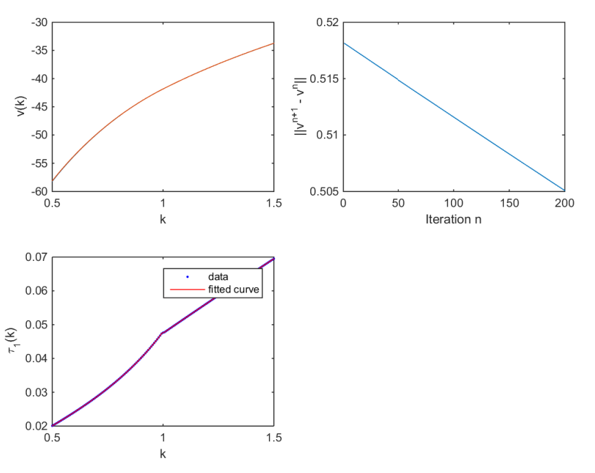
I used a CB Production function $f(k)=k^\alpha$ with $Ak$-Technology, that is $f(k)=k$ (for $\alpha<1$ I have a problem) and log preferences a la $u(g,c)=\ln g +c$. A linear cost function with $a:\theta\mapsto (1-\theta)$. I stopped after 200 iterations which already lasted for 21mins. In the first panel is the guess of the 1st and 200th value function. The second panel shows the difference for between the value function (convergence tendency). And the last panel ist the actual policy function, say, $\tau_1(k)$ (note the kink at $k=1=k^*$). It seems to be right from an intuitive perspective. That is, a country lowers its tax rate on capital if the capital stock is realitively small and vive versa. I'm not quite sure why the procedure is so time consuming.
test

Update

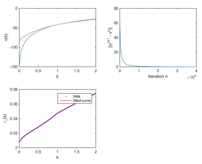
I was able to increase the speed. Then I increased the range of the grid to the respective endpoints of the state, as well as the number of grid points and ran the VFI (40000 Iterations) until I was out of memory. First panel contains first and final value function. The algorithms is converging with $|v^{40000}-v^{39999}|=0.0077$. The kink in the policy function still remains, but the shape slightly differs now. test2
$\endgroup$
1
  • $\begingroup$ You need way too many iterations, I never needed more than, say, 20. Are you using the implicit method? Whats your $\Delta$? $\endgroup$
    – FooBar
    Commented Apr 15, 2015 at 17:15

1 Answer 1

3
$\begingroup$

I don't think I've seen cases with a kink in continuous time that are solved numerically. Aguiar & Amador (2014) have a kink in their HJB, but they solve their HJB analytically.

Validation

I don't know to what extent Moll et al's algorithm is going to get that right. You will most likely get weird behavior around the kink, but whether it's the real functional form is to be doubted, and you'll have to argue ex-post that "it looks okay alright?".

If you want to get a better grip into whether the kink looks alright, make it more extreme. Without going through your equations, it seems that the first part is convex and the second part is linear. Increase the curvature for the first part so you can "see" more easily whether it still looks correct around the kink.

Also, you definitively should look at the numerical counterparts to the first-order and second-order derivative, the first-order and second-order difference of the approximation divided by the step size. Do they have the correct signs around the kink?

One thing I'd emphasize is having many grid points around the kink. However, since the algorithm gets tougher when you have a nonlinear grid (because the grid step size is now not a constant, but a vector), it might just not be worth it and you could rather jack up overall grid points and keep it linear.

Speed

Finally, you really should look into having sparse matrices for the A and B matrices. 10 iterations per minute is really slow. It takes you perhaps 30 minutes to understand and implement (if you've never worked with sparse systems before), but already after the second time you run the code you've made up that time.

If the problem persists, have a look at profilers for your coding language. For Python, this is a nice solution. Even if you have everything sparse, perhaps you forgot some matrix that you don't even need in the iteration loop. That was the case for me, and with large grid sizes that single reinitialization took up a lot of time. Profiler will tell you what's what.

$\endgroup$
4
  • $\begingroup$ Concerning speed: I am using matlab. I define functions within the script. For example I have for the utility function, which is seperated at the fixed point, the following functions U1_1(k, tau1, tau2) = log(k*tau1) + f(k) - k*tau1 + C1(k, tau2); U1_2(k, tau1) = log(k*tau1) + f(k) + df(k)*(1-k) - tau1; where previously $f(k)$ and its derivatives are defined as f(k) = k^a; df(k) = diff(f,k);. Then in the iteration loop I use u1(1:iss-1) = U1_1(k(1:iss-1), tau1(1:iss-1), tau2(1:iss-1)); u1(iss:I) = U1_2(k(iss:I), tau1(iss:I)); where k(iss)=1$=k^*$. Should I use extra function files? $\endgroup$
    – clueless
    Commented Apr 15, 2015 at 5:43
  • $\begingroup$ General Question: What's the deal and major difference between defining f(k)=k^a at the beginning of your working script work.mor save an extra function fun.m file which contains function y = f(k) y = k^a; and call it within work.m whenever needed. $\endgroup$
    – clueless
    Commented Apr 15, 2015 at 5:51
  • $\begingroup$ @clueless you should look at a profiler to evaluate what's slowing you down most. I used to work with Matlab, and there it was the rule, that every single initialization of functions was coming with an overhead, s.t. you'd want to not call functions within loops because you'd lose much efficiency. However, I've heard that that's better now, and also, you iterate much less with this method than with ordinary Value-Function iteration. $\endgroup$
    – FooBar
    Commented Apr 15, 2015 at 11:12
  • $\begingroup$ The major difference is one of style. Having your functions in a separate file and loading that makes your main file clearer to read and more structured. $\endgroup$
    – FooBar
    Commented Apr 15, 2015 at 11:13

Your Answer

By clicking “Post Your Answer”, you agree to our terms of service and acknowledge you have read our privacy policy.

Not the answer you're looking for? Browse other questions tagged or ask your own question.