2
$\begingroup$

In lecture, my professor defined the following 2-period consumption model:

$c_i = $ consumption in period $i$.

$y =$ endowed income in period 1.

$r = $ interest rate in perfect credit markets.

$h = $ money invested in period 1.

$w(h) = $ period 2 return on money invested in period 1.

$U(c_1, c_2) = u(c_1) + \beta u(c_2)$ an additively separable utility function with discount factor $\beta$.

Then the budget constraint is $$c_1 + \frac{c_2}{1+r} = y - h + \frac{w(h)}{1+r}$$ so the Lagrangian for utility maximization is $$L = u(c_1) + \beta u(c_2) + \lambda \left( y - h + \frac{w(h)}{1+r} - c_1 - \frac{c_2}{1+r} \right).$$ But then $h^*$ is determined entirely by one of the first order conditions, $$L_h = \frac{w'(h)}{1+r} - 1 = 0,$$ which is independent of $\beta$.

My professor said that this means "patient and impatient people invest the same amount $h^*$, maximizing the net present value of income." Mathematically, I understand why this has to be true, but intuitively it doesn't make sense. If $\beta = 0$, for example, shouldn't we invest $h=0$ because all consumption in the future provides 0 utility? Why doesn't similar reasoning apply to very small $\beta$? And why would we be trying to maximize the NPV of income if income in the first period provides more utility than income in the second period?

$\endgroup$

2 Answers 2

4
$\begingroup$

This idea is known as the Fisher separation theorem.

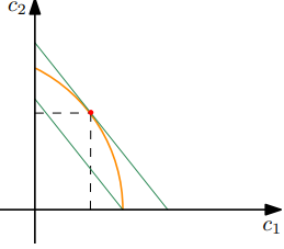
Without the investment opportunity to transfer $h$ units of present day value into $w(h)$ units of future value, the perfect credit market gives us the intertemporal budget constraint of $$ c_1 + \frac{c_2}{1+r} = y, $$ which can be represented by a straight line.

enter image description here

Without knowledge of the consumer's preferences, it is not possible to say what the optimal $(c_1,c_2)$ is here. But we can say with certainty, that the higher the budget line is, the more options the consumer has, and assuming monotonic preferences she will be better off.

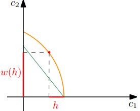
Now the yield curve $w$ of the investment opportunity allows us to shift the basic credit market budget line. Starting from the lower right point of $(y,0)$ (i.e. not putting money into the credit market at all) we can reach cash flows $(y-h, w(h))$.

enter image description here

But by also putting some money into the credit market (or borrowing), one can reach other cash flows as well. These always transfer $x$ units of present value into $x(1+r)$ units of future value (in case of borrowing $x$ is negative), so they are always paralel to the original budget line, but instead of starting from $(y,0)$, they start from the point $(y-h, w(h))$ where $h$ is the size of the investment.

The optimal investment size is the one that reaches the highest budget line:

enter image description here


The idea is that given perfect credit markets one can separate consumption behavior and investment behavior. The higher the net present value of my cash flow, the better of I will be once I adjust my cash flow via the credit market to my intertemporal preferences (this is where $\beta$ matters). Thus I need to make investment decisions that maximize the present value of my cash flow, and I do not have to take anything else into consideration, e.g., the timing of the payments.


A mathematical tidbit:

In the above example, given the optimal $h$ (assuming it is an interior point) the budget line is tangential to the orange curve depicting the possible investments, so we have $$ w'(h) = 1 + r, $$ the marginal yield from the investment and the credit market are equal. This is equivalent to the final equation in your question.

$\endgroup$
0
$\begingroup$

Well i just edited my answer a lot. I made a fundamentally mistake, from $ L_ {h} $ arises an unique value of h, even when $ h $ is in other first order conditions, that doesn't change anything. Once that i have clear that there is no relationship between $ \beta $ and $ h $, I think I know what is happening.

The reason why it is invested in $ h $ although $ \beta = 0 $ is because h increases the NPV, and this allows to increase consumption in the first period. What happens is $\beta=0 \ \Rightarrow \ \ c_{2}=0$. But let´s see this more carefully.

To do this we have to add restrictions to the model $c_{1},c_{2},h > 0$, so the lagrangian will change:

\begin{align} L= L = u(c_1) + \beta u(c_2) + \lambda_{1} \left( y - h + \frac{w(h)}{1+r} - c_1 - \frac{c_2}{1+r} \right) +\lambda_{2}c_{1}+\lambda_{3}c_{2}+\lambda_{4}h \end{align}

The new first order conditions will be:

\begin{align} \frac{\partial L}{\partial c_{1}} = u^{ ' }(c_{1}) - \lambda_{1} + \lambda_{2} =0 \ (1)\\ \frac{\partial L}{\partial c_{2}} = \beta u^{ '}(c_{2}) - \frac{\lambda_{1}}{1+r} + \lambda_{3}=0 \ (2)\\ \frac{\partial L}{\partial h} =(\frac{ w^{ ' }(h)}{1+r} -1)\lambda_{1} + \lambda_{4}= 0 \ (3)\\ \end{align}

But we need for constraints with inequalities the complementary slackness conditions (we can work with the Kuhn-Tucker lagrangian, but that it's just a special case of this general formulation):

\begin{align} \lambda_{1}(y-h + \frac{ w(h)}{1+r} - \frac{ c_{2}}{1+r}-c_{1}) =0 \ (4) \\ \lambda_{2}(c_{1})=0 \ (5) \\ \lambda_{3}(c_{2})=0 \ (6) \\ \lambda_{4}(h)=0 \ (7) \\ \end{align}

This means that either the restriction or the $\lambda_{i}$ will be 0. To solve this equations we need to exhaust all posibilities, and see if we can arrive to a solution that is consistent or discard cases that lead to contradiction. Im going to show that $\beta=0 \ \Rightarrow \ c_{2}=0, \ h=constant$. You can look for yourself to check if there is other posible solutions.

So let's see if $\beta=0 \ \Rightarrow \ c_{2}=0, \ h=constant$ it's a solution. if $\beta=0$ the logical thing would be to think that the optimal solution would be $c_{2}^{*}=0$, so let's just assume that this it's the case, if it is not, at some point the first order conditions must show that this is not consistent.

Also, we expect that $c_{1}>0$ which implies by (5) $\lambda_{2}=0$. We can see from (1) that $\lambda_{1}>0$ because the assumption $u(c_{i})>0$. Now, here comes the interesting part if $\frac{w^{'}(h^{*})}{1+r}-1>0$ implies that $\lambda_{4}=0$ by (3). Not always this would be the case, for example suppose that $w(h)=h(1+v)$ where $v$ is the return of investment in $h$. $\frac{w^{'}(h^{*})}{1+r}-1$ would be $ \frac{v-r}{1+r}$. If $v>r$ then $\frac{w^{'}(h^{*})}{1+r}-1>0$ and $\lambda_{4}=0$. But if $v<r$ then $\lambda_{4}>0$ by (3) and $h=0$ by (7).

This means that the optimal choice of h depends on this condition. If the return of h is bigger that his cost of oportunity (including r), then $h>0$ and would be a constant.

Now let's rule out the posibility that $c_{2}>0$. If this is true, $\lambda_{3}=0$, which by (2) implies that $\lambda_{1}=0$, which implies by (1) that $u^{'}(c_{1})=0$ that generally it's not true. So our assumption that $c_{2}^{*}=0$ it's in general correct.

So all this observations lead us to the following equations:

\begin{align} u^{ ' }(c_{1}) = \lambda_{1} \ (8)\\ \lambda_{1}=(1+r)\lambda_{3} \ (9)\\ \frac{ w^{ ' }(h)}{1+r} = 1 \ (10)\\ c_{1}^{*} = y-h + \frac{ w(h)}{1+r} - \frac{1}{1+r} (11) \end{align}

(8) comes from (1), (9) from (2), (10) from (3), and (11) from (4). From this system of equations the solutions to all the endogenous variables are obtained for $c_{1}^{*}$ is (11) and for $h$ is (10). So $\beta=0 \ \Rightarrow \ c_{2}=0$. Why $h_{*}>0$? This happens because investing in $h$ increases the NPV, so increases the consumption today, so invest in h increases utility in period 1.This does not depend on $\beta$, because it's a monetary relationship. But note that if the return of $r$ is greater thatn $h$, then it could happen that $h^{*}=0$.

$\endgroup$
12
  • $\begingroup$ You seem to be talking about savings, not investment. $\endgroup$
    – Giskard
    Commented Jun 28, 2020 at 7:09
  • $\begingroup$ Yes, because you save to invest in h or to consume in period two. $\endgroup$ Commented Jun 28, 2020 at 7:20
  • $\begingroup$ If it's not clear that the dependence exists. You can just substitute the restriction on the utility function for some $c_{i}$ and derivate for $h$ and $c_{2}$, and it's more clear that a dependence exists. Or just choose some utility function and solve it. $\endgroup$ Commented Jun 28, 2020 at 7:24
  • $\begingroup$ $h$ appears in two first order conditions, you need to solve them to see of what depends $h$ $\endgroup$ Commented Jun 28, 2020 at 7:26
  • $\begingroup$ Unless I misunderstand the model, "investing" is not the only way to make money in period 2, you can also put your money into the "perfect credit market". Otherwise the discount factor $1/(1+r)$ makes little sense. Thus savings would equal the invested sum $h$ plus the amount of money earning interest in this market. $\endgroup$
    – Giskard
    Commented Jun 28, 2020 at 9:43

Your Answer

By clicking “Post Your Answer”, you agree to our terms of service and acknowledge you have read our privacy policy.

Not the answer you're looking for? Browse other questions tagged or ask your own question.