How do I correctly incorporate a $3 tax on supply to each unit sold?

Question

I am wondering how to properly add a $3 tax on supply to each unit sold. I have done a welfare analysis pre tax to the following equations:

Demand: $Q = 400-2P$
Supply: $Q = 3P + 50$

When adding the tax I believe I should see an increase in equilibrium price but if I change the supply equation accordingly:

Supply $Q = 3(P+3) + 50$

When I solve for the equilibrium price it goes from 70 to 68.8. Should I be doing:

Supply $Q = 3(P-3) + 50$

I am trying to do some simple welfare analyses but getting stuck at this part, any help would be greatly appreciated!

Answer 1

You first solve for $P$ in the supply curve.

$Q = 3P + 50 \iff 3P = Q - 50$

$\iff P = \frac{Q}{3} - \frac{50}{3}$.

Since the producers got taxed, they need to charge a higher price to cover their costs (The right hand side of $P =$ can be interpreted as the minimum amount of money producers are willing to accept for selling the $Q$-th unit):

$P^t = \frac{Q}{3} - \frac{50}{3} + 3$

Simplifying,

$P^t = \frac{Q}{3} - \frac{41}{3}$

This is the new supply curve after including the tax.

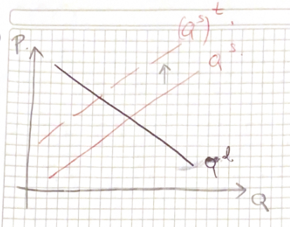
Adding that $3$ to the right hand side of $P=$ corresponds to shifting the supply curve upwards, which due to the upward sloping nature of the curve, it is equivalent to a left shift (for a given market price, less units are supplied).

Graphically, we have this situation:

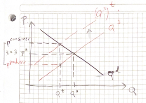
Which causes this new equilibrium:

In presence of a tax, the prices perceived by the consumer and the producer aren’t the same anymore, now you need to find both prices.

As a rule of thumb, in presence of a tax, $P^{\text{consumer}} > P^\star > P^{\text{producer}}$, and $Q^t < Q^\star$.

On the other hand, in presence of a subsidy, the reverse happens.

To find the new equilibrium quantity, you equate demand and taxed supply.

I get $Q^t = 256.4 < 260 = Q^\star$

Plugging into demand (or equivalently as seen on the graph, plugging into taxed supply) you get the price perceived/paid by the consumer:

I get $P^{\text{consumer}} = 71.8 > 70 = P^\star$.

Since both prices have to differ by the tax amount,

$P^{\text{producer}} = P^{\text{consumer}} - 3 = 71.8 - 3 = 68.8 < 70 = P^\star$.

The price you actually got is the price perceived/earned by the producer, which goes down as expected. The price that goes up is the price paid by the consumer, you have to remember you are now searching for two prices.

Since the consumer pays a higher price and the producer earns a lower price, they are both worse off with the tax.

Answer 2

the subscript $d$ denote demand and $s$ denote supply. Using this notation let us rewrite the demand and supply functions.

Demand function before tax: $Q_d(P_d)=400-2P_d \quad \dots (1)$
Supply function before tax: $Q_s(P_s)=3P_s+50 \quad \;\quad \dots (2)$

Before-tax equilibrium price is: $P_d=P_s=70$

Now, a tax of $t=3$ per unit is imposed on the good.
This gives us the relation: $P_s+t=P_d \iff P_s=P_d-t$

we can modify $(1)$ and $(2)$ as functions of $P_d$ and solve for equilibrium by equating market demand and market supply

At equilibrium: $$\begin{eqnarray} Q_d(P_d)=Q_s(P_d-t)\\ 400-2P_d=3(P_d-3)+50 \\ 400-2P_d=3P_d-3t+50 \\ P_d=71.8 \end{eqnarray}$$

Therefore, the after-tax equilibrium price is: $P=71.8$ which is higher than the before-tax equilibrium price.