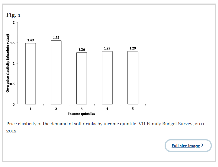
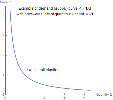
Basically, you're correct that elasticity is a summary statistic under the assumption that the curve "looks like" an ideal demand/supply curve, i.e one with constant elasticity. This assumption is usually pretty valid, e.g. here's empirical data estimating the elasticity of the demand of soft drink across incomes groups (quintiles):

In general, (in the math-sense) the (point) elasticity of a function is itself a function, which may or may be constant, but it is so for the "usual" demand curves:
The elasticity of a function is a constant $\alpha$ if and only if the function has the form $f(x) = C x ^ \alpha$ for a constant $C>0$.

The elasticity at a point is the limit of the arc elasticity between two points as the separation between those two points approaches zero.
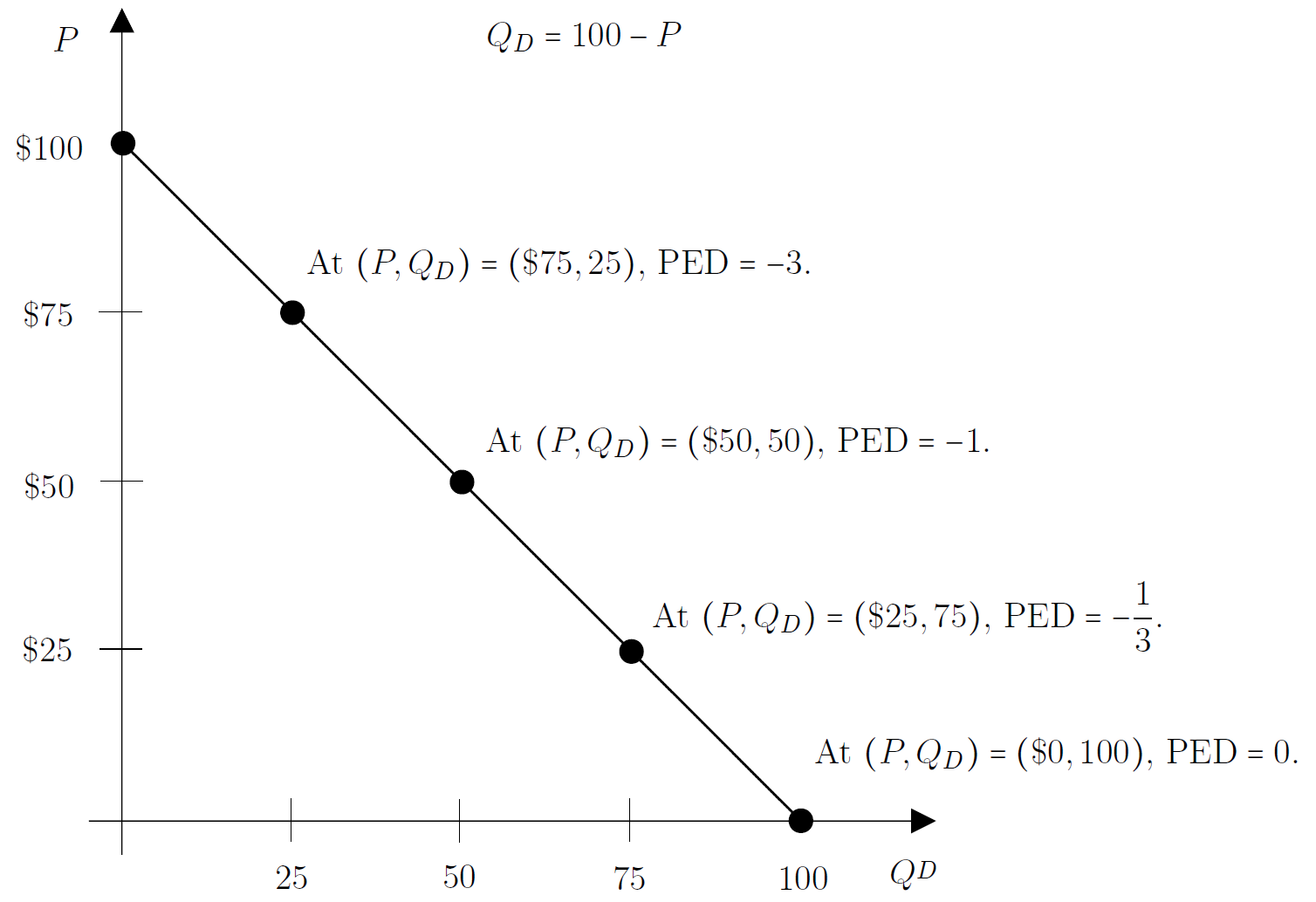
Finally the bit you said about "elastic and inelastic" regions is a bit of a confusion, as it's not about an elasticity curve itself in separation, but rather
On a graph with both a demand curve and a marginal revenue curve, demand will be elastic at all quantities where marginal revenue is positive. Demand is unit elastic at the quantity where marginal revenue is zero. Demand is inelastic at every quantity where marginal revenue is negative
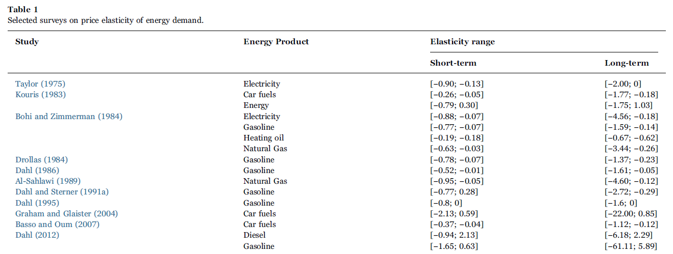
Per [expert] protest below, an expert answer should say that estimating elasticities is a fairly difficult problem (for the obvious reason that we don't get to experience all the price points).
almost all price-elasticities which are presented in the literature are estimated on macro timeseries data by means of demand systems under Slutsky constraints. They are generally considered as being not robust to the specification of the demand system and they suffer from aggregation biases and lack of information on price variations. Moreover the stationarity conditions are generally rejected for long-term time-series.
Second, estimation technics on cross-section individual data (such as surveys on consumer expenditures) are either based on separability assumptions over the utility function (Frisch, 1959, Deaton, 1974) which allows to calculate price elasticities in terms of income elasticities and the Frisch’s income flexibility (see Theil, 1986, Selvanathan, 1993), or on unit values
(ratio of the value of expenditures over the corresponding quantities whenever both are recorded in the survey, generally for food expenditures, see Deaton, 1988). The first method is based on the assumption of strong separability which generally is not supported by the data. The second concerns only those rare datasets which contain both values and quantities of
consumption, generally only for food commodities.
Third, arc-elasticity can be computed between two periods (see Gardes, Merrigan, 2011
for such an estimation for tobacco). In contrast to estimation on macro data, this method
allows to compute price effects for different types of households, but it necessitates
comparable repeated cross-sections or a panel over a period characterized by large price
changes. Moreover, it concerns only the direct price effect for the commodity having
experienced this price change.
A fourth method consists in computing semi-aggregate price indexes for a set of products
using the individual budget shares as a weight of the individual product prices: these
aggregate prices are thereby individualized and can be used to estimate price elasticities on a
cross-section survey. This method initiates in remarks by Hicks and Stone and was fully
discussed by Lewbel (1989). It has been recently applied by Ruiz and Trannoy (2007) on the
French Household Expenditures surveys and proved efficient, but perhaps not very robust
(considering the volatility of estimates in Ruiz’s thesis, 2006). Those techniques imply the
endogeneity of semi-aggregate prices (since they are defined by means of current budget
shares) which can be corrected by instrumentation. More critical is the assumption that the set
of detailed commodities (such as various durables for home cleaning) are sufficiently
different to experience different price changes, but pertain to a homogenous group as
concerns households’ preferences: whenever they differ sufficiently, the difference in the
composition of the corresponding aggregate for two households implies that the semiaggregate does not play the same role in these households’ consumption, and thus the price
change of the semi-aggregate is largely due to a change in its composition or quality. The
hidden assumption of that method (commodities within an aggregate consumption play the
same role in the household’s consumption) is thus intrinsically illogical: either the
commodities are similar, and their prices must follow the same trend; or they differ, and the
role of the aggregate in household’s consumption depends on the proportion of the detailed
commodities in this aggregate.
The kind of empirical graph I showed you as empirical "evidence" is based on the 2nd kind of method, if I'm not mistaken.
